quality analysis of water

# Type at least 1 character to search # Hit enter to search or ESC to close

No products in the cart.

Product Categories

• New Products
• Dissolved Oxygen
• Conductivity
• Temperature
• Oxygen (gas)
• Atlas Iot - Raspberry Pi Software
• AtlasDesktop
• Dosing Pumps
• Flow Meters
• Float Switches
• Probe Mounting
• EZO-Complete
• Waterproofing
• Carrier Boards
• Calibration Solutions
• Electrical Isolation
• Embedded Solutions
• EZO™ Accessories

Featured Products

• Distributors
• Calculators
• Privacy Policy
• Return Policy

A Complete Guide To Water Analysis Methods In Industries

• November 3, 2023

Share This Post

Water analysis refers to the process of testing and evaluating the quality of water. It involves examining various physical, chemical, and biological properties to determine the quality of water. These results help to identify any potential health risks or environmental concerns associated with the water source being analyzed. 

Water analysis is a vital process used to assess the quality and composition of water. It is a critical step to ensure that water is safe and clean for drinking, industrial use, agriculture, and aquatic ecosystems, just to name a few. The water analysis process involves measuring various parameters (like pH, conductivity, etc) and contaminants present in the water to ensure its safety for consumption and suitability for specific applications. 

What Is The Need For Water Analysis Methods?

One of the main reasons why water analysis is important is to ensure that the water we consume on a daily basis, is safe for drinking. Contaminated water can pose serious health risks, as the water may contain harmful bacteria, viruses, chemicals, or heavy metals. Therefore, if we conduct regular water analysis, we can identify any potential threats and take appropriate measures to treat or filter the water and improve the quality, before it reaches our taps. This is particularly vital for more vulnerable people such as children, pregnant women, and people who have compromised immune systems. These people are typically more susceptible to waterborne diseases.

Water analysis is also essential for environmental monitoring and protection. By analyzing the water in rivers, lakes, and oceans, scientists and environmentalists can assess the health of aquatic ecosystems and identify any pollutants or contaminants that may be affecting aquatic life. This information helps in planning effective conservation and management strategies to preserve these fragile ecosystems.

Water analysis also provides valuable data for research purposes, such as studying various aspects of water quality and its impact on different ecosystems and species. This data helps in understanding the long-term effects/trends, identifying emerging contaminants, and developing new technologies or treatment methods to address water-related challenges.

The Importance Of Water Analysis Methods In Industries

Water analysis methods are crucial for a wide range of industries that rely on water for their operations, like the food and beverage industry . In this industry, water is used extensively in daily operations, such as cleaning, cooking, and ingredient preparation. Therefore, it is essential to analyze the quality of water at different points along the process to ensure that it meets the required standards for consumption and production. By completing a water analysis, you can detect any contaminants or impurities that may affect the taste, safety, and overall quality of the final product(s).

Another industry that heavily relies on water analysis methods is the pharmaceutical industry . Water is a critical component in the manufacturing of pharmaceutical products, including drugs and vaccines in equipment such as bioreactors . The purity and quality of water used in these processes are of utmost importance to ensure the safety of the end products. 

The agriculture industry is also heavily dependent on water analysis methods. Irrigation is a vital stage in agriculture, and therefore, water quality plays a significant role in crop growth and yield. Analyzing the water used for irrigation helps pinpoint any harmful substances, such as pesticides or heavy metals, that may be present in the water. This allows farmers to take appropriate measures to mitigate any negative impacts on their crops, ensure the safety of their produce, and prevent contaminating surrounding areas from surface runoff. 

Additionally, power generation and oil refineries require water analysis methods to monitor the quality of water used for cooling systems and steam generation. Contaminants in water can easily lead to corrosion, scaling, and fouling of equipment, which can result in reduced efficiency and increased maintenance costs. Therefore, regular water analysis is essential to maintain smooth operations and follow safety precautions. 

Types Of Water Analysis Methods

Water quality analysis is a practice that involves examining the properties and parameters of water to ensure its safety and cleanliness. 

Chemical Water Analysis Methods

Chemical analysis is a fundamental part of water quality analysis. It requires testing for different chemical parameters to identify contaminants and assess their levels in water. Some of the commonly tested chemical parameters include ammonia, chloride ion, nitrite, nitrate, phosphate, and water hardness.

Chloride Ion: The concentration of chloride ions in water can indicate contamination levels and the potential presence of saline water. High chloride ion levels can lead to a salty taste in water and may cause corrosion in water pipelines. These not only negatively affect the quality of water, but they can also incur higher maintenance costs.

Ammonia: Ammonia is often a byproduct of organic matter decomposition and can often be found in water sources. Ammonia concentrations increase with the use of chloramine in water disinfection processes. High levels of ammonia in drinking water can have adverse health effects, and its presence may lead to distinctive tastes and odors.

Nitrite & Nitrate: Nitrite and nitrate are forms of nitrogen that can be found in water due to organic matter decomposition and atmospheric nitrogen fixation. Nitrite can be toxic, especially in high concentrations, and can cause health issues such as “blue baby syndrome” in infants. Nitrate, on the other hand, enhances the growth of aquatic plants and can contribute to water eutrophication in natural water systems, where excessive plant growth in ponds and lakes takes place. 

Phosphate: Phosphate is present in water in various forms, including dihydrogen phosphate (H2PO4-), polyphosphate (polyP), and organic phosphate. Phosphate fundamentally comes from agricultural waste, sewage, and industrial effluents. While phosphate itself is not toxic, high concentrations can lead to water eutrophication.

Hardness: Water hardness refers to the presence of calcium and magnesium salts in water. Temporary hardness is caused by carbonate and bicarbonate ions, while permanent hardness is due to chloride and sulfate ions. Hard water can have certain benefits for drinking purposes, but excessive levels of certain ions can be a nuisance because of scale buildup. 

Physical Water Analysis Methods

Physical analysis of water involves assessing its various physical properties, such as temperature, color, turbidity, and conductivity. These parameters provide valuable information about the clarity and suitability of water for various purposes.

Temperature: Water temperature plays a significant role in various physical and biological processes as it affects the dissolved oxygen content, the solubility of gases, and the growth of aquatic organisms. Temperature measurements are simple, yet essential for understanding the overall health and functioning of aquatic ecosystems.

Color: The color of the water can indicate the presence of suspended or dissolved substances. Apparent color refers to the color caused by suspended matter, while true color is caused by dissolved solids. Also, excessive color in water can be aesthetically unpleasant and may indicate the presence of organic compounds that can interfere with disinfection processes.

Turbidity: Turbidity is important as it measures the extent to which light is absorbed or scattered by suspended particles in water . It indicates the presence of particulate matter, such as sediment (like soil), algae, or organic particles, and can easily be measured with a turbidity meter . The problem with high turbidity levels is that high turbidity can affect the aesthetics of water and cause issues with disinfection processes.

Conductivity: Conductivity measures the ability of water to conduct an electrical current, which is influenced by the presence of dissolved salts, minerals, and other ions. The greater the number of ions, the higher the conductivity level . Conductivity provides insights into the overall mineral content and salinity of water and its suitability for various applications and industries.

Biological Water Analysis Methods

Biological analysis focuses on assessing the presence of microorganisms and other biological indicators in water. These indicators can provide an understanding of the overall health and safety of the water. A good example is bacteria testing.

Bacteria testing is essential in determining the safety and potability (suitability for drinking) of water. One of the most common bacteria tested for is E. coli, which is an indicator of fecal contamination. High levels of E. coli in water can indicate the presence of harmful pathogens that can pose serious health issues when consumed. Bacteria testing helps in identifying potential microbial contamination like E.coli and ensures the safety of water for drinking and other uses.

The Role Of Water Testing Laboratories

Water testing laboratories have a crucial role in water quality analysis. These specialized facilities are equipped with advanced instruments and trained personnel to perform a wide range of tests and analyses. Laboratories provide environments that ensure accurate and reliable results, which are essential for making informed decisions regarding water management and treatment.

Water testing laboratories also offer a comprehensive suite of tests, and follow standardized protocols and quality control measures to ensure the accuracy and precision of their results. Water analysis labs therefore can provide expert guidance and interpretation of the data obtained to help industries understand the implications of poor water quality and take appropriate actions.

Water Analysis: Understanding Analytical Methods

Analytical methods are procedures designed to measure the concentration of specific contaminants in water samples. These methods provide a structure for collecting, preserving, and storing samples, in addition to separating, identifying, and quantifying contaminants. Analytical methods also establish quality control criteria and outline the reporting standards.

Analytical methods serve many purposes, including demonstrating regulation compliance, meeting monitoring objectives, and providing data for water samples that require routine analysis. These methods typically have upper and lower limits within which the concentration of drinking water contaminants should be. They also incorporate quality control measures to ensure accurate and reliable results.

Development & Evaluation Of Water Analysis Methods

Abbreviations:

• ASTM: American Society for Testing & Materials
• DIN: German Institute of Norms
• EN: European Unions
• EPA: Environmental Protection Agency (US)
• ISO: International Organization for Standardization
• SCA: Standing Committee of  Analysts (Blue Books)
• SLMB: Swiss Book for the Analysis of Food
• USP: United State Pharmacopoeia 

Analytical methods used in water analysis are developed by various organizations, including governmental bodies like the EPA, consensus method organizations such as Standard Methods and ASTM International, universities, water labs, and commercial distributors. 

The EPA evaluates methods developed by others through its Alternate Test Procedure Program . This program assesses the accuracy, precision, and reliability of analytical methods from different sources.

EPA approval of methods occurs when regulating new contaminants or through other rulemaking actions. The accelerated approval process is employed to streamline the approval of drinking water analytical methods. Laboratories supporting public water systems are required to use EPA-approved methods for analyzing samples to demonstrate compliance with drinking water regulations.

Major Parameters & Corresponding Water Analysis Methods

Water analysis encompasses the measurement of various parameters and contaminants. Below are some of the most common parameters that are analyzed and the corresponding analytical methods.

Electrical Conductivity

Electrical conductivity is a key parameter used to assess the salinity and total dissolved solids in water. It provides insights into the water’s ability to conduct an electric current. 

Several standard methods are employed to determine electrical conductivity in water samples, including ASTM D 1125 , EPA 120.1, ISO 7888, DIN EN 27888, and USP 645. 

The pH value of water indicates its acidity or alkalinity and is an essential parameter to assess water quality . 

ASTM D 5464, EPA 150.2, DIN EN ISO 10523, SCA 14, and SLMB 602.1 are some of the standard methods used to measure the pH value of water. 

Fluoride is a naturally occurring mineral that, when present at excessive levels, can have detrimental effects on human health. The analysis of fluoride in water samples is crucial to ensure that its concentration falls within acceptable limits. 

ASTM D 1179, ASTM D 3868, DIN 38405-4, EPA 340.2, ISO 10359-1, SCA 62, and SLMB 626.1 are some of the standard methods employed for fluoride analysis.

Ammonium & Total Kjeldahl Nitrogen

Ammonium and Total Kjeldahl nitrogen (TKN) are parameters used to assess the presence of nitrogen compounds in water samples. They provide insights into the levels of organic and inorganic nitrogen in water, which can indicate pollution and potential health risks. 

ASTM D 1426, ASTM D 3590, DIN 38406-5, EPA 350.2, EPA 350.3, EPA 351.3, EPA 351.4, ISO 5663, ISO 5664, ISO 6778, SCA 126, and SLMB 631.1 are some of the standard methods employed for the analysis of ammonium and TKN. 

Ion Chromatography

Ion chromatography is a widely used technique for the analysis of anions and cations in water samples. It involves the separation and quantification of various ions, providing insights into the chemical composition of the water. 

ASTM D 4327, ASTM D 5085, ASTM D 5257, ASTM D 5542, ASTM D 5996, ASTM D 6581, ASTM D 6919, EPA 218.6, EPA 300.0, EPA 300.1, EPA 314.0, EPA 317.0, DIN EN ISO 10304-1, DIN EN ISO 10304-3, DIN EN ISO 10304-4, DIN EN ISO 14911, DIN EN ISO 15061, SCA 631.1, and SLMB 658.1 are some of the standard methods employed for ion chromatography. 

Instrumental Methods Used In Labs

Apart from the field-testing methods, instrumental methods are used in laboratory settings to analyze water samples. These methods employ sophisticated electronic instrumentation to measure trace levels of contaminants and provide rapid and accurate results.

• Ion chromatography: Measures trace levels of anions
• Atomic absorption spectroscopy, inductively coupled ion spectroscopy, and x-ray fluorescence spectroscopy: Detects trace levels of different elements
• Gas chromatography: Used to quantify volatile compounds 
• High-pressure liquid chromatography: Used to separate and detect trace organic compounds in antimicrobial systems
• Total organic carbon: Used to determine the number of organics in water where leaks or organic fouling of resins has occurred
• Nuclear magnetic resonance spectroscopy: Used to evaluate the structure of organic polymers and other water treatment chemicals
•  Fourier-transform infrared analysis: Used to identify and quantify the composition of boiler and cooling system deposits

How To Prepare & Collect Samples For Water Analysis

To ensure accurate and meaningful results, proper sample collection and preparation are essential in water analysis.

Firstly, it’s important to understand the different methods of water analysis. Various tests and parameters can be measured, such as pH level, dissolved oxygen, turbidity, and the presence of contaminants like bacteria or heavy metals. Depending on the specific analysis you want to perform, you should select the appropriate method and collect the sample accordingly.

To start with, make sure you have the necessary equipment before collecting water samples. You will need clean and sterile bottles or containers to avoid contamination. It’s recommended to use glass or high-quality plastic containers that are specifically designed for water sampling. You should also have gloves, a waterproof marker, and labels to properly identify and record the samples.

Next, it’s important to choose the correct sampling location. The location should be representative of the water source you are analyzing. For example, if you are testing the quality of tap water in your home, you should collect the sample directly from the tap. If you are analyzing water from a river or lake, choose a spot that is away from any potential sources of contamination, such as industrial areas or sewage outlets.

When collecting the water sample, always take precautions to minimize any potential contamination. Start by rinsing the sampling container thoroughly with the same water source you are collecting from. This helps remove any impurities or residues that may affect the analysis results. Then, carefully fill the container without allowing it to touch any surfaces or come into contact with your hands.

It’s important to collect enough water for the analysis. The amount required may vary depending on the specific test or analysis method. Generally, it’s recommended to collect at least 500 milliliters (ml) of water for most standard tests. However, for more comprehensive analyses or if you need multiple tests done, you may need larger samples.

After collecting the sample, ensure that it is properly labeled and recorded. Labeling should include important information such as the location, date, and time of collection. This information is crucial for accurate data interpretation and comparison with future analyses.

Finally, take proper care of the collected samples until they reach the laboratory for analysis. Keep them in a cool and dark place to minimize any potential changes in their properties. If possible, transport them in a cooler with ice packs to maintain their temperature during transit.

Samples should be cooled to room temperature before testing, typically ranging from 21-26°C (70-80°F) – a temperature of 25°C is recommended for the majority of water analysis methods . Filtration through 0.2-2.5 µm filters may be necessary to remove particulate matter and ensure the purity of the sample.

Water Collection Methods

One common method for collecting water samples is the grab sampling technique . This involves using a clean container, such as a glass bottle or a plastic bag, to directly collect a sample of water from a specific source. 

It is important to choose a container that is free from any contaminants that could alter the composition of the water being collected. To ensure accuracy, it is recommended to collect multiple grab samples from different locations within the water source. This helps to account for any variations in water quality that may exist across the area being sampled.

Another method for collecting water samples is the composite sampling technique . This involves collecting multiple grab samples over a specific period, usually 24 hours, and combining them into one representative sample. 

The purpose of composite sampling is to obtain an average composition of the water over a given period. This method is often used when monitoring water quality over an extended period or when testing for contaminants that may fluctuate throughout the day.

Water analysis methods play a vital role in assessing the quality and safety of water for various applications. By employing standardized water analytical methods, industries can ensure accurate and reliable results, promoting the overall health and well-being of communities and ecosystems.

If you have any questions regarding water quality analysis, or what water quality testing kits we offer, do not hesitate to contact the world-class team at Atlas Scientific . 

Conductivity Probes & Circuits

pH Probes & Sensors

Subscribe To Our Newsletter

Get product updates and learn from the best, more to explore.

How to calibrate the EZO Complete-TMP using the Atlas Desktop software

The Atlas Scientific line of EZO Complete circuits makes building a custom monitoring system easy, but if you don’t calibrate your sensors, then what good are your readings; And can you trust them? The accuracy of your readings is directly related to the quality of your calibration. Calibration is not difficult, and a little bit

Want to learn more about our products?

Atlas scientific | all rights reserved © 2024.

To track your order please enter your Order ID in the box below and press the "Track" button. This was given to you on your receipt and in the confirmation email you should have received.

Billing email

• Close Email Address Password Show password Forgot your password? Sign In Create an account

Choose your country or region:

• België /Belgique
• Česká Republika
• Deutschland
• Magyarország
• United Kingdom

Asia - Australasia

• Mainland China
• New Zealand
• Philippines
• South Korea (한국)
• Thailand (ไทย)
• América Latina
• United States

Middle East - Africa

• Middle East & North Africa
• East, Central & West Africa
• South and Southern Africa
• Ships Next Day
• Claros Portal
• Worldwide Locations
• Order Status
• Express Order

Successfully added to cart

Water Analysis Handbook

The Water Analysis Handbook (WAH) is the result of more than 85 years of research and method development. With over 300 illustrated, step-by-step instructions, this is your comprehensive source for water analysis procedures. From instruments to reagents, meters to probes, media to general lab supply, this handbook outlines everything you need to perform each procedure, simplifying the water analysis process.

WAH Downloads

Abbreviations and Conversions Table Common in Written Chemical Procedures

Acid-Base, Acid and Base Determination Method 8200 and Method 8233

Acid-Base, Sodium Hydroxide for meq/L of Acid; Sulfuric Acid for meq/L of Base. Method 8288 and Method 8289

Acidity for Water, Wastewater and Seawater

Acidity, Methyl Orange-Sodium Hydroxide with a Buret Method 8219

Acidity, Methyl orange and Phenolphthalein (Total) Acidity-Method 8201 and Method 8202

Acidity, Phenolphthalein-Sodium Hydroxide with a Buret Method 8010

Alkalinity for Water, Wastewater and Seawater

Alkalinity, Buret Titration Method 8221

Alkalinity, Phenolphthalein and Total Alkalinity Method 8203

Alkalinity, Total, Colorimetric Method, TNTplus™ 870, Method 10239

Aluminum Aluminon Method 8012

Aluminum Chromazurol S Method 10215

Aluminum PP Method 8326

Aluminum for Water

Arsenic Silver Dientyldithiocarbamate Method 8013

Atrazine Immunoassay Method 10050

Bacteria Membrane Filtration Method, Pre-poured Agar Plate

Bacteria Test Guidelines

Bacteria, Hydrogen Sulfide Producing, Presence/Absence Method 8506

Bacteria, Hydrogen Sulfide Producing-Most Probable Number Method 10032

Barium Turbidimeter Method 8014

Barium for Water, Wastewater, Oil-field water and Seawater

Benzotriazole and Tolyltriazole for Water

Benzotriazole/Tolyltriazole UV Photolysis Method 8079

Boron Azomethine-H Method LR

Boron Carmine Method 8015

Boron for Water and Wastewater

Bromine DPD Method 8016

Cadmium Cadion Method 10217

Cadmium Dithizone Method 8017

Carbon Dioxide for Water and Seawater

Carbon Dioxide, Buret titration Method 8223

Carbon Dioxide, Digital Titrator using Sodium Hydroxide Method 8205

Chelant, Free-Digital Titrator using Magnesium Chloride Method 8352

Chelant, Total-Bismuth Nitrate Method 8350

Chemical Analysis

Chemical Oxygen Demand for Wastewater

Chemical Oxygen Demand, Mn III for Water and Wastewater

Chloramine (Mono) Indophenol Method 10171

Chloramine (Mono) Indophenol Method 10172

Chloramine (Mono); Free Ammonia Method 10200

Chloride Mercuric Thiocyanate Method 8113

Chloride for Water and Wastewater

Chloride, Mercuric Nitrate Method 8206

Chloride, Silver Nitrate Buret Titration Method 8225

Chloride, Silver Nitrate Method 8207

Chlorine Demand/Requirement, DPD Reagent Method 10223

Chlorine Dioxide Chlorophenol Red method 8065

Chlorine Dioxide DPD Method 10126

Chlorine Dioxide Direct Reading Method 8138

Chlorine Dioxide Direct Reading Method 8345

Chlorine Dioxide for Water and Wastewater

Chlorine, Free DPD Method 10069

Chlorine, Free DPD Method 8021

Chlorine, Free DPD Rapid Liquid Method 10059

Chlorine, Free DPD TNT Method 10102

Chlorine, Free MR, USEPA DPD Method 10245

Chlorine, Free and Total TNTplus™, DPD Method. Free Chlorine: Method 10231; Total Chlorine: Method 10232

Chlorine, Free and Total for Water, Wastewater and Seawater

Chlorine, Free and Total-DPD-FEAS Method 8210

Chlorine, Free, Indophenol Method 10241

Chlorine, Free-Amperometric Buret Titration Method 8334

Chlorine, Free-Amperometric Forward Titration, Method 10024

Chlorine, Hypochlorite-Iodometric HR Method 10100

Chlorine, Total DPD Method 10014

Chlorine, Total DPD Method 10070

Chlorine, Total DPD Method 8167

Chlorine, Total DPD Method 8370

Chlorine, Total DPD Rapid Liquid Method 10060

Chlorine, Total DPD TNT Method 10101

Chlorine, Total- DPD, MR, Method 10250

Chlorine, Total-Amperometric Back Titration Method 10025

Chlorine, Total-Amperometric Buret Titration Method 8168

Chlorine, Total-Amperometric Forward Titration, Method 10026

Chlorine, Total-Iodometric Method 8161

Chlorine, Total-Iodometric using Sodium Thiosulfate Method 8209

Chromate, Titration using Sodium Thiosulfate Method 8211

Chromium for Water and Wastewater

Chromium, Hexavalent Method 8023

Chromium, Hexavalent-1,5-diphenylcarbohydrazide Method 10218. Chromium, Total-1,5-Diphenylcarbohydrazide Method 10219

Chromium, Total Alkaline Hypobromite Oxidation Method 8024

Cobalt 1-(2-Pyridylazo)-2-Naphthol (PAN) Method 8078

Cobalt for water

Coliforms, Presence/Absence-P/A Broth Method 8319. P/A Broth with MUG Method 8364

Coliforms-E. coli, Membrane Filtration (modified m-TEC) Method 8367

Coliforms-E. coli, Membrane Filtration Method 8367

Coliforms-Fecal, A-1 Medium, Most Probable Number (MPN) Method 8368

Coliforms-Fecal, Membrane Filtration (m-FC and m-FC/RA) Method 8074

Coliforms-Total and E. coli, Membrane Filtration Method 10029

Coliforms-Total and E.coli, Lauryl Tryptose with MUG Broth, Most Probable Number (MPN) Method 8091

Coliforms-Total, Fecal and E.coli, Lauryl Tryptose Broth, Most Probable Number (MPN) Method 8001

Coliforms-Total, Fecal and E.coli, Lauryl Trypyose Broth, Most Probable Number Method 8001A

Coliforms-Total, Fecal and E.coli-Membrane Filtration, m-Endo, Method 8074

Color, ADMI-ADMI Weighted Ordinate Method 10048

Color, True & Apparent, Platinum-Cobalt Standard Method 8025

Color, True and Apparent, Low Range, Platinum-Cobalt Standard Method (8025)

Conductivity, Direct Measurement Method 8160

Copper Bicinchoninate Method 8506 and Method 8026

Copper Porphyrin Method 8143

Copper for Water, Wastewater and Seawater

Copper, Bathocuproine Method, TNTplus™ 860, Method 10238

Cyanide Pyridine-Pyrazalone Method 8027

Cyanide for Water, Wastewater and Seawater

Cyanuric Acid, Turbidimetric Method 8139

Definitions of USEPA Approved and Accepted

Direct Measurement ISE, TISAB Solution, Method 8359

Dissolved Oxygen HRDO HR Method 8166

Dissolved Oxygen Indigo Carmine LR Method 8316

Dissolved Oxygen Ultra High Range Method 8333

Dissolved Oxygen for Water, Wastewater, and Seawater

Dissolved Oxygen, Azide Modification of Winkler Method 8215 and Method 8332

Dissolved Oxygen, Direct Measurement, Clark-type Amperometric Sensor, Method 8157

Dissolved Oxygen, Direct Measurement, LDO Probe, Method 10360

Dissolved Oxygen-Azide Modification of Winkler Method 8229

Enterococci (Coliforms) Membrane Filtration, Proposed Method 1600

Fluoride SPADNS Method 8029

Fluoride for Water and Seawater

Fluoride in Acid Solutions, Direct Measurement ISE Electrode Method 8323

Fluoride in Drinking Water, Direct Measurement ISE, Powder Pilow or TISAB Solution, Method 8323

Fluoride, SPADNS 2 Method 10225

Formaldehyde MBTH Method 8110

Formaldehyde for Water

No resources available at this time.

Hardness Calcium & Magnesium; Calmagite Colorimetric Method 8030

Hardness Calcium & Magnesium; Chlorophosphonazo Colorimetric Method 8374

Hardness for Water, Wastewater and Seawater

Hardness, Calcium-Buret Titration Method 8222

Hardness, Calcium-Titration Method using EDTA Method 8204

Hardness, Total Sequential-Buret Titration Method 8338

Hardness, Total, Sequential, Titration using EDTA, Method 8329

Hardness, Total-Calcium & Magnesium Chlorophosphonazo Rapid Liquid Method 8374

Hardness, Total-ManVer 2 Buret Titration Method 8226

Hardness, Total-Titration using EDTA Method 8213

Heterotrophic Bacteria, Membrane Filtration Method, m-TGE Broth with TTC Indicator-Method 8242

Heterotrophic Bacteria, Membrane Filtration Method, m-TGE Broth, Method 8242

Heterotrophic Bacteria, Membrane Filtration, m-HPC, Method 8242

Heterotrophic Bacteria, Membrane Filtration, m-TSB-USP, Method 8242

Heterotrophic Bacteria, Pour Plate, Plate Count Agar, Method 8241

Heterotrophic Bacteria, Pour Plate, m-HPC, Method 8242

Heterotrophic Bacteria, Pour Plate, m-TGE with TTC, Method 8242

Heterotrophic Bacteria, Pour Plate, m-TGE, Method 8242

Heterotrophic Bacteria, Pour Plate, m-TSB/USP, Method 824

Hydrazine for Water and Boiler Water

Hydrazine p-Dimethylaminobenzaldehyde Method 8141

International Guideline Comparison between International Drinking Water and FDA Bottled Water

Iodine DPD Method 8031

Iron FerroZin ® Rapid Liquid Method 8147

Iron Ferrozine Method 8147

Iron for Water and Seawater

Iron, Ferrous 1-10 Phenanthroline Method 8146

Iron, TNTplus™ 858, Phenanthroline Method 10229

Iron, TitraVer Titration Method 8214

Iron, Total FerroMo Method 8365

Iron, Total FerroVer ® Method 8008

Iron, Total TPTZ Method 8112

Laboratory Practices

Langelier and Agressive Indices for Method 8073

Lead Dithizone Method 8033

Lead LeadTrak™ Fast Column Extraction Method 8317

Lead PAR Method 10216

Lead for Water and Wastewater

MPN (Most Probable Number) Dilution Guidelines

Manganese 1-(2-Pyridylazo)-2-Naphthol PAN Method 8149

Manganese Periodate Oxidation Method 8034

Manganese for Water and Wastewater

Membrane Filtration Guidelines

Mercury Cold Vapor Mercury Concentration Method 10065

Mercury, Cold Vapor

Molybdenum Mercaptoacetic Acid Method 8036

Molybdenum Ternary Complex Method 8169

Molybdenum, Molybdate for Water

Monochloramine for Water and Wastewater

Monochloramine; Nitrogen, Free Ammonia

Nickel 1-(2-Pyridylazo)-2-Napthol (PAN) Method 8150

Nickel Dimethylglyoxime Method 10220

Nickel Heptoxime Method 8037

Nickel for Water

Nitrate Cadmium Reduction LR Method 8192

Nitrate Cadmium Reduction Method 8039

Nitrate Cadmium Reduction Method 8171

Nitrate Chromotropic Acid TNT Method 10020

Nitrate Dimethylphenol HR Method 10206

Nitrate UV Screening Method 10049

Nitrate, Dimethylphenol LR Method 10206

Nitrate, Direct Measurement ISE, Powder Pillow or TISAB Solution, Method 8358

Nitrite Diazotization LR Method 10019

Nitrite Diazotization LR Method 10207

Nitrite Diazotization LR Method 8507

Nitrite Ferrous Sulfate HR Method 8153

Nitrite, Ceric Acid Titration Method 8351

Nitrite, Diazotization, HR, TNTplus™ Method 10237

Nitrogen Total Inorganic-Titanium Trichloride Reduction Method 10021

Nitrogen Total Kjeldahl-Nessler Method 8075

Nitrogen Total-Persulfate Digestion HR Method 10208

Nitrogen, Ammonia for Water, Wastewater and Seawater

Nitrogen, Ammonia-Direct Measurement ISE Electrode, Method 10001

Nitrogen, Ammonia-Known Addition ISE Electrode, Method 10002

Nitrogen, Ammonia-Nessler Method 8038

Nitrogen, Ammonia-Salicylate HR Method 10031

Nitrogen, Ammonia-Salicylate HR TNT Method 10205

Nitrogen, Ammonia-Salicylate LR TNT Method 10023

Nitrogen, Ammonia-Salicylate LR TNT Method 10205

Nitrogen, Ammonia-Salicylate Method 8155

Nitrogen, Ammonia-Salicylate ULR TNT Method 10205

Nitrogen, Free Ammonia-Indophenol Method 10201

Nitrogen, Kjeldahl for Water and Wastewater

Nitrogen, Nitrate for Water and Wastewater

Nitrogen, Nitrite for Water and Wastewater

Nitrogen, Simplified TKN (s-TKN™), Method 10242

Nitrogen, Total for Water, Wastewater and Seawater

Nitrogen, Total-Persulfate Digestion HR Method 10072

Nitrogen, Total-Persulfate Digestion LR Method 10071

Nitrogen, Total-Persulfate Digestion LR TNT Method 10208

Nitrogen, Total-Persulfate Digestion UHR TNT Method 10208

Oil and Grease, Solid Phase Extraction Method 10300

Oli and Grease Hexane Extractable Gravimetric Method 10056

Organic Carbon, Total-Direct LR Method 10129

Organic Carbon, Total-HR Direct Method 10128

Organic Carbon, Total-MR Direct Method 10173

Organic Constituents UV Absorbing (UV-254), Direct Reading Method 10054

Organic Constituents, UV Transmission (UV-254), Direct Reading Method 10243

Oxidation Reduction Potential (ORP), Direct Measurement-ORP Electrode-Method 10228

Oxygen Demand, Biochemical, Dilution LBOD Measurement, Method 10230

Oxygen Demand, Biochemical-Dilution Method 8043

Oxygen Demand, Chemical, Mercury-Free Reactor Digestion, TNTplus™ 825, Method 10236

Oxygen Demand, Chemical-Manganese III Reactor Digestion Method 10067 (with Chloride Removal)

Oxygen Demand, Chemical-Manganese III Reactor Digestion Method 10067 (without Chloride Removal)

Oxygen Demand, Chemical-Reactor Digestion Method 8000

Oxygen Demand, Chemical-Reactor Digestion Method 8000, TNTPlus™

Oxygen Demand, Chemical-Reactor Digestion ULR TNT Method 10211

Oxygen Demand, Chemical-UHR Reactor Digestion Method 10212

Oxygen Scavengers Iron Reduction Method 8140

Oxygen Scavengers for Water

Ozone Indigo Method 8311

Ozone for Water

Peracetic Acid (PAA) 1 and Hydrogen Peroxide (H 2 O 2 )

pH, Electrode Method 8156

pH Indicators for Water and Wastewater

Phenols 4-Aminoantipyrine Method 8047

Phenols for Water, Wastewater, and Seawater

Phosphonates Persulfate UV Oxidation Method 8007

Phosphonates for Water

Phosphorus for Water, Wastewater and Seawater

Phosphorus, Acid Hydrolyzable Digestion-Acid Digestion Method 8180

Phosphorus, Acid Hydrolyzable-PhosVer™ 3 with Acid Hydrolysis TNT Method 8180

Phosphorus, Reactive (Orthophosphate) Amino Acid Method 8178

Phosphorus, Reactive (Orthophosphate) Molybdovanadate Method 10214

Phosphorus, Reactive (Orthophosphate) Molybdovanadate Method 8114

Phosphorus, Reactive (Orthophosphate) Molybdovanadate TNT Method 8114

Phosphorus, Reactive (Orthophosphate) PhosVer ® TNT Method 8048

Phosphorus, Reactive (Orthophosphate) and Total-Ascorbic Acid, TNTplus™ 843, LR Method 10209 (Reactive) and Method 10210 (Total)

Phosphorus, Reactive (Orthophosphate) and Total-Ascorbic Acid, TNTplus™ 844, Method 10209 (Reactive) and Method 10210 (Total)

Phosphorus, Reactive (Orthophosphate) and Total-Ascorbic Acid, TNTplus™ 845, UHR Method 10209 (Reactive) and Method 10210 (Total)

Phosphorus, Reactive (Orthophosphate)-PhosVer 3 (Ascorbic Acid) Method 8048

Phosphorus, Reactive-Ascorbic Acid Rapid Liquid LR Method 10055

Phosphorus, Reactive-Molybdovanadate Rapid Liquid HR Method 8114

Phosphorus, Total Molybdovanadate Method with Acid Persulfate Digestion HR TNT Method 10127

Phosphorus, Total, Digestion-Acid Persulfate Digestion Method 8190

Phosphorus, Total-PhosVer ® with Acid Persulfate Digestion TNT Method 8190

Potassium Tetraphenylborate Method 8049

Potassium for Water and Wastewater

Pseudomonas (Coliform), Membrane Filtration Method 8026

Quaternary Ammonium Compounds-Direct Binary Complex Method 8337

Salinity, Mercuric Nitrate Method 10073

Sample Pretreatment by Digestion

Selenium Diaminobenzidine Method 8194

Selenium for Water and Wastewater

Silica Heteropoly Blue ULR Method 8282

Silica for Water and Seawater

Silica-Heteropoly Blue LR Method 8186

Silica-Heteropoly Blue Rapid Liquid ULR Method 8282

Silica-Silicomolybdate HR Method 8185

Silver, Colorimetric Method 8120

Sodium, Direct Measurement ISE Electrode, Method 8359

Solids, Nonfilterable Suspended Solids; Total and Volatile-Gravimetric Method 8158 and Method 8164

Solids, Settleable Matter-Direct Measurement Method 8165

Solids, Total Filterable (Total Dissolved Solids), Gravimetric Method 8163

Solids, Total Volatile and Fixed-Gravimetric Method 8276

Solids, Total-Gravimetric Method 8271

Solids, Volatile Dissolved and Fixed Dissolved-Gravimetric Method 8277

Sulfate SulfaVer 4 Method 8051

Sulfate for Water, Seawater and Oil-field Water

Sulfate, Turbidimetric, TNTplus™ 864, Method 10227

Sulfate, Turbidimetric, TNTplus™ 865, Method 10227

Sulfide Methylene Blue Method 8131

Sulfide for Water, Wastewater and Seawater

Sulfite for Water, Wastewater and Seawater

Sulfite, Iodate-Iodide Buret Titration Method 8071

Sulfite, Iodate-Iodide Method 8216

Surfactants, Anionic (Detergents)-Crystal Violet Method 8028

Suspended Solids, Photometric Method 8006

Tannin and Lignin Tyrosine Method 8193

Total Aerobic Bacteria, Yeasts and Molds-Paddle Testers

Total Organic Carbon for Water and Wastewater

Total Petroleum Hydrocarbons (TPH) Immunoassay Method 10050

Toxicity, ToxTrak™ Method 10017

Trihalomethane Formation Potential (THMFP) THM Plus Method 10224

Trihalomethanes, THM Plus™ Method 10132

Volatile Acids, Buret Titration Method 8291

Volatile Acids, Esterification Method 8196

Volatile Acids, Esterification, TNTplus™ 872, Method 10240

Volatile Acids, Sodium Hydroxide Method 8218

Water Management and Safety

Water Analysis Guide (includes an application guide, abbreviations and conversions, lab practices, chemical analysis, sample pretreatment by digestion, bacteria analysis, and waste management/safety)

Zinc for Water and Wastewater

Zinc, Zincon Method 8009

Open Access is an initiative that aims to make scientific research freely available to all. To date our community has made over 100 million downloads. It’s based on principles of collaboration, unobstructed discovery, and, most importantly, scientific progression. As PhD students, we found it difficult to access the research we needed, so we decided to create a new Open Access publisher that levels the playing field for scientists across the world. How? By making research easy to access, and puts the academic needs of the researchers before the business interests of publishers.

We are a community of more than 103,000 authors and editors from 3,291 institutions spanning 160 countries, including Nobel Prize winners and some of the world’s most-cited researchers. Publishing on IntechOpen allows authors to earn citations and find new collaborators, meaning more people see your work not only from your own field of study, but from other related fields too.

Brief introduction to this section that descibes Open Access especially from an IntechOpen perspective

Want to get in touch? Contact our London head office or media team here

Our team is growing all the time, so we’re always on the lookout for smart people who want to help us reshape the world of scientific publishing.

Home > Books > Water Quality - Science, Assessments and Policy

Water Quality Parameters

Submitted: 15 August 2019 Reviewed: 10 September 2019 Published: 16 October 2019

DOI: 10.5772/intechopen.89657

Cite this chapter

There are two ways to cite this chapter:

From the Edited Volume

Water Quality - Science, Assessments and Policy

Edited by Kevin Summers

To purchase hard copies of this book, please contact the representative in India: CBS Publishers & Distributors Pvt. Ltd. www.cbspd.com | [email protected]

Chapter metrics overview

14,721 Chapter Downloads

Impact of this chapter

Total Chapter Downloads on intechopen.com

Total Chapter Views on intechopen.com

Overall attention for this chapters

Since the industrial revolution in the late eighteenth century, the world has discovered new sources of pollution nearly every day. So, air and water can potentially become polluted everywhere. Little is known about changes in pollution rates. The increase in water-related diseases provides a real assessment of the degree of pollution in the environment. This chapter summarizes water quality parameters from an ecological perspective not only for humans but also for other living things. According to its quality, water can be classified into four types. Those four water quality types are discussed through an extensive review of their important common attributes including physical, chemical, and biological parameters. These water quality parameters are reviewed in terms of definition, sources, impacts, effects, and measuring methods.

• water quality
• physical parameters
• chemical parameters
• biological parameters
• radioactive substances
• toxic substances
• indicator organisms

Author Information

Nayla hassan omer *.

• Department of Environmental Engineering, College of Water and Environmental Engineering, Sudan University for Science and Technology, Khartoum, Sudan

*Address all correspondence to: [email protected]

1. Introduction

Water is the second most important need for life to exist after air. As a result, water quality has been described extensively in the scientific literature. The most popular definition of water quality is “it is the physical, chemical, and biological characteristics of water” [ 1 , 2 ]. Water quality is a measure of the condition of water relative to the requirements of one or more biotic species and/or to any human need or purpose [ 3 , 4 ].

2. Classification of water

Based on its source, water can be divided into ground water and surface water [ 5 ]. Both types of water can be exposed to contamination risks from agricultural, industrial, and domestic activities, which may include many types of pollutants such as heavy metals, pesticides, fertilizers, hazardous chemicals, and oils [ 6 ].

Potable water: It is safe to drink, pleasant to taste, and usable for domestic purposes [ 1 , 7 ].

Palatable water: It is esthetically pleasing; it considers the presence of chemicals that do not cause a threat to human health [ 7 ].

Contaminated ( polluted) water: It is that water containing unwanted physical, chemical, biological, or radiological substances, and it is unfit for drinking or domestic use [ 7 ].

Infected water: It is contaminated with pathogenic organism [ 7 ].

3. Parameters of water quality

There are three types of water quality parameters physical, chemical, and biological [ 8 , 9 ]. They are summarized in Table 1 .

3.1 Physical parameters of water quality

3.1.1 turbidity.

Turbidity is the cloudiness of water [ 10 ]. It is a measure of the ability of light to pass through water. It is caused by suspended material such as clay, silt, organic material, plankton, and other particulate materials in water [ 2 ].

It can increase the cost of water treatment for various uses [ 11 ].

The particulates can provide hiding places for harmful microorganisms and thereby shield them from the disinfection process [ 12 ].

Suspended materials can clog or damage fish gills, decreasing its resistance to diseases, reducing its growth rates, affecting egg and larval maturing, and affecting the efficiency of fish catching method [ 13 , 14 ].

Suspended particles provide adsorption media for heavy metals such as mercury, chromium, lead, cadmium, and many hazardous organic pollutants such as polychlorinated biphenyls (PCBs), polycyclic aromatic hydrocarbons (PAHs), and many pesticides [ 15 ].

The amount of available food is reduced [ 15 ] because higher turbidity raises water temperatures in light of the fact that suspended particles absorb more sun heat. Consequently, the concentration of the dissolved oxygen (DO) can be decreased since warm water carries less dissolved oxygen than cold water.

Turbidity is measured by an instrument called nephelometric turbidimeter, which expresses turbidity in terms of NTU or TU. A TU is equivalent to 1 mg/L of silica in suspension [ 10 ].

Turbidity more than 5 NTU can be visible to the average person while turbidity in muddy water, it exceeds 100 NTU [ 10 ]. Groundwater normally has very low turbidity because of the natural filtration that occurs as the water penetrates through the soil [ 9 , 16 ].

3.1.2 Temperature

Palatability, viscosity, solubility, odors, and chemical reactions are influenced by temperature [ 10 ]. Thereby, the sedimentation and chlorination processes and biological oxygen demand (BOD) are temperature dependent [ 11 ]. It also affects the biosorption process of the dissolved heavy metals in water [ 17 , 18 ]. Most people find water at temperatures of 10–15°C most palatable [ 10 , 19 ].

3.1.3 Color

Materials decayed from organic matter, namely, vegetation and inorganic matter such as soil, stones, and rocks impart color to water, which is objectionable for esthetic reasons, not for health reasons [ 10 , 20 ].

Color is measured by comparing the water sample with standard color solutions or colored glass disks [ 10 ]. One color unit is equivalent to the color produced by a 1 mg/L solution of platinum (potassium chloroplatinate (K 2 PtCl 6 )) [ 10 ].

Apparent color is the entire water sample color and consists of both dissolved and suspended components color [ 10 ].

True color is measured after filtering the water sample to remove all suspended material [ 19 ].

Color is graded on scale of 0 (clear) to 70 color units. Pure water is colorless, which is equivalent to 0 color units [ 10 ].

3.1.4 Taste and odor

Taste and odor in water can be caused by foreign matter such as organic materials, inorganic compounds, or dissolved gasses [ 19 ]. These materials may come from natural, domestic, or agricultural sources [ 21 ].

The numerical value of odor or taste is determined quantitatively by measuring a volume of sample A and diluting it with a volume of sample B of an odor-free distilled water so that the odor of the resulting mixture is just detectable at a total mixture volume of 200 ml [ 19 , 22 ]. The unit of odor or taste is expressed in terms of a threshold number as follows:

where TON is the threshold odor number and TTN is the threshold taste number.

3.1.5 Solids

Solids occur in water either in solution or in suspension [ 22 ]. These two types of solids can be identified by using a glass fiber filter that the water sample passes through [ 22 ]. By definition, the suspended solids are retained on the top of the filter and the dissolved solids pass through the filter with the water [ 10 ].

If the filtered portion of the water sample is placed in a small dish and then evaporated, the solids as a residue. This material is usually called total dissolved solids or TDS [ 10 ].

freshwater: <1500 mg/L TDS;

brackish water: 1500–5000 mg/L TDS;

saline water: >5000 mg/L TDS.

The residue of TSS and TDS after heating to dryness for a defined period of time and at a specific temperature is defined as fixed solids. Volatile solids are those solids lost on ignition (heating to 550°C) [ 10 ].

Total solids:

Interrelationship of solids found in water [ 22 ].

Total dissolved solids:

Total suspended solids:

Fixed and volatile suspended solids:

where VSSA = weight of residue + dish and filter before ignition, mg and VSSB = weight of residue + dish and filter after ignition, mg.

3.1.6 Electrical conductivity (EC)

The electrical conductivity (EC) of water is a measure of the ability of a solution to carry or conduct an electrical current [ 22 ]. Since the electrical current is carried by ions in solution, the conductivity increases as the concentration [ 10 ] of ions increases. Therefore, it is one of the main parameters used to determine the suitability of water for irrigation and firefighting.

U.S. units = micromhos/cm

S.I. units = milliSiemens/m (mS/m) or dS/m (deciSiemens/m)

Ultra-pure water: 5.5 × 10 −6  S/m;

Drinking water: 0.005–0.05 S/m;

Seawater: 5 S/m.

The electrical conductivity can be used to estimate the TDS value of water as follows [ 10 , 22 ]:

TDS can be used to estimate the ionic strength of water in the applications of groundwater recharging by treated wastewater [ 22 ]. The normal method of measurement is electrometric method [ 10 ].

3.2 Chemical parameters of water quality

pH is one of the most important parameters of water quality. It is defined as the negative logarithm of the hydrogen ion concentration [ 9 , 12 ]. It is a dimensionless number indicating the strength of an acidic or a basic solution [ 23 ]. Actually, pH of water is a measure of how acidic/basic water is [ 19 , 20 ]. Acidic water contains extra hydrogen ions (H + ) and basic water contains extra hydroxyl (OH − ) ions [ 2 ].

As shown in Figure 2 , pH ranges from 0 to 14, with 7 being neutral. pH of less than 7 indicates acidity, whereas a pH of greater than 7 indicates a base solution [ 2 , 24 ]. Pure water is neutral, with a pH close to 7.0 at 25°C. Normal rainfall has a pH of approximately 5.6 (slightly acidic) owing to atmospheric carbon dioxide gas [ 10 ]. Safe ranges of pH for drinking water are from 6.5 to 8.5 for domestic use and living organisms need [ 24 ].

pH of water.

A change of 1 unit on a pH scale represents a 10-fold change in the pH [ 10 ], so that water with pH of 7 is 10 times more acidic than water with a pH of 8, and water with a pH of 5 is 100 times more acidic than water with a pH of 7. There are two methods available for the determination of pH: electrometric and colorimetric methods [ 10 ].

Excessively high and low pHs can be detrimental for the use of water. A high pH makes the taste bitter and decreases the effectiveness of the chlorine disinfection, thereby causing the need for additional chlorine [ 21 ]. The amount of oxygen in water increases as pH rises. Low-pH water will corrode or dissolve metals and other substances [ 10 ].

Pollution can modify the pH of water, which can damage animals and plants that live in the water [ 10 ].

Most aquatic animals and plants have adapted to life in water with a specific pH and may suffer from even a slight change [ 15 ].

Even moderately acidic water (low pH) can decrease the number of hatched fish eggs, irritate fish and aquatic insect gills, and damage membranes [ 14 ].

Water with very low or high pH is fatal. A pH below 4 or above 10 will kill most fish, and very few animals can endure water with a pH below 3 or above 11 [ 15 ].

Amphibians are extremely endangered by low pH because their skin is very sensitive to contaminants [ 15 ]. Some scientists believe that the current decrease in amphibian population throughout the globe may be due to low pH levels induced by acid rain.

Heavy metals such as cadmium, lead, and chromium dissolve more easily in highly acidic water (lower pH). This is important because many heavy metals become much more toxic when dissolved in water [ 21 ].

A change in the pH can change the forms of some chemicals in the water. Therefore, it may affect aquatic plants and animals [ 21 ]. For instance, ammonia is relatively harmless to fish in neutral or acidic water. However, as the water becomes more alkaline (the pH increases), ammonia becomes progressively more poisonous to these same organisms.

3.2.2 Acidity

Acidity is the measure of acids in a solution. The acidity of water is its quantitative capacity to neutralize a strong base to a selected pH level [ 10 ]. Acidity in water is usually due to carbon dioxide, mineral acids, and hydrolyzed salts such as ferric and aluminum sulfates [ 10 ]. Acids can influence many processes such as corrosion, chemical reactions and biological activities [ 10 ].

Carbon dioxide from the atmosphere or from the respiration of aquatic organisms causes acidity when dissolved in water by forming carbonic acid (H 2 CO 3 ). The level of acidity is determined by titration with standard sodium hydroxide (0.02 N) using phenolphthalein as an indicator [ 10 , 20 ].

3.2.3 Alkalinity

The alkalinity of water is its acid-neutralizing capacity comprised of the total of all titratable bases [ 10 ]. The measurement of alkalinity of water is necessary to determine the amount of lime and soda needed for water softening (e.g., for corrosion control in conditioning the boiler feed water) [ 22 ]. Alkalinity of water is mainly caused by the presence of hydroxide ions (OH − ), bicarbonate ions (HCO 3− ), and carbonate ions (CO 3 2− ), or a mixture of two of these ions in water. As stated in the following equation, the possibility of OH − and HCO 3 − ions together are not possible because they react together to produce CO 3 2− ions:

Alkalinity is determined by titration with a standard acid solution (H 2 SO 4 of 0.02 N) using selective indicators (methyl orange or phenolphthalein).

The high levels of either acidity or alkalinity in water may be an indication of industrial or chemical pollution. Alkalinity or acidity can also occur from natural sources such as volcanoes. The acidity and alkalinity in natural waters provide a buffering action that protects fish and other aquatic organisms from sudden changes in pH. For instance, if an acidic chemical has somehow contaminated a lake that had natural alkalinity, a neutralization reaction occurs between the acid and alkaline substances; the pH of the lake water remains unchanged. For the protection of aquatic life, the buffering capacity should be at least 20 mg/L as calcium carbonate.

3.2.4 Chloride

Chloride occurs naturally in groundwater, streams, and lakes, but the presence of relatively high chloride concentration in freshwater (about 250 mg/L or more) may indicate wastewater pollution [ 7 ]. Chlorides may enter surface water from several sources including chloride-containing rock, agricultural runoff, and wastewater.

Chloride ions Cl − in drinking water do not cause any harmful effects on public health, but high concentrations can cause an unpleasant salty taste for most people. Chlorides are not usually harmful to people; however, the sodium part of table salt has been connected to kidney and heart diseases [ 25 ]. Small amounts of chlorides are essential for ordinary cell functions in animal and plant life.

Sodium chloride may impart a salty taste at 250 mg/L; however, magnesium or calcium chloride are generally not detected by taste until reaching levels of 1000 mg/L [ 10 ]. Standards for public drinking water require chloride levels that do not exceed 250 mg/L. There are many methods to measure the chloride concentration in water, but the normal one is the titration method by silver nitrate [ 10 ].

3.2.5 Chlorine residual

Chlorine (Cl 2 ) does not occur naturally in water but is added to water and wastewater for disinfection [ 10 ]. While chlorine itself is a toxic gas, in dilute aqueous solution, it is not harmful to human health. In drinking water, a residual of about 0.2 mg/L is optimal. The residual concentration which is maintained in the water distribution system ensures good sanitary quality of water [ 11 ].

Chlorine can react with organics in water forming toxic compounds called trihalomethanes or THMs, which are carcinogens such as chloroform CHCl 3 [ 11 , 22 ]. Chlorine residual is normally measured by a color comparator test kit or spectrophotometer [ 10 ].

3.2.6 Sulfate

Sulfate ions (SO 4 2− ) occur in natural water and in wastewater. The high concentration of sulfate in natural water is usually caused by leaching of natural deposits of sodium sulfate (Glauber’s salt) or magnesium sulfate (Epson salt) [ 11 , 26 ]. If high concentrations are consumed in drinking water, there may be objectionable tastes or unwanted laxative effects [ 26 ], but there is no significant danger to public health.

3.2.7 Nitrogen

There are four forms of nitrogen in water and wastewater: organic nitrogen, ammonia nitrogen, nitrite nitrogen, and nitrate nitrogen [ 10 ]. If water is contaminated with sewage, most of the nitrogen is in the forms of organic and ammonia, which are transformed by microbes to form nitrites and nitrates [ 22 ]. Nitrogen in the nitrate form is a basic nutrient to the growth of plants and can be a growth-limiting nutrient factor [ 10 ].

A high concentration of nitrate in surface water can stimulate the rapid growth of the algae which degrades the water quality [ 22 ]. Nitrates can enter the groundwater from chemical fertilizers used in the agricultural areas [ 22 ]. Excessive nitrate concentration (more than 10 mg/L) in drinking water causes an immediate and severe health threat to infants [ 19 ]. The nitrate ions react with blood hemoglobin, thereby reducing the blood’s ability to hold oxygen which leads to a disease called blue baby or methemoglobinemia [ 10 , 19 ].

3.2.8 Fluoride

A moderate amount of fluoride ions (F − ) in drinking water contributes to good dental health [ 10 , 19 ]. About 1.0 mg/L is effective in preventing tooth decay, particularly in children [ 10 ].

Excessive amounts of fluoride cause discolored teeth, a condition known as dental fluorosis [ 11 , 19 , 26 ]. The maximum allowable levels of fluoride in public water supplies depend on local climate [ 26 ]. In the warmer regions of the country, the maximum allowable concentration of fluoride for potable water is 1.4 mg/L; in colder climates, up to 2.4 mg/L is allowed.

There are four methods to determine ion fluoride in water; the selection of the used method depends on the type of water sample [ 10 ].

3.2.9 Iron and manganese

Although iron (Fe) and manganese (Mn) do not cause health problems, they impart a noticeable bitter taste to drinking water even at very low concentration [ 10 , 11 ].

These metals usually occur in groundwater in solution as ferrous (Fe 2+ ) and manganous (Mn 2+ ) ions. When these ions are exposed to air, they form the insoluble ferric (Fe 3+ ) and manganic (Mn 3+) forms making the water turbid and unacceptable to most people [ 10 ].

These ions can also cause black or brown stains on laundry and plumbing fixtures [ 7 ]. They are measured by many instrumental methods such as atomic absorption spectrometry, flame atomic absorption spectrometry, cold vapor atomic absorption spectrometry, electrothermal atomic absorption spectrometry, and inductively coupled plasma (ICP) [ 10 ].

3.2.10 Copper and zinc

Copper (Cu) and zinc (Zn) are nontoxic if found in small concentrations [ 10 ]. Actually, they are both essential and beneficial for human health and growth of plants and animals [ 25 ]. They can cause undesirable tastes in drinking water. At high concentrations, zinc imparts a milky appearance to the water [ 10 ]. They are measured by the same methods used for iron and manganese measurements [ 10 ].

3.2.11 Hardness

Hardness is a term used to express the properties of highly mineralized waters [ 10 ]. The dissolved minerals in water cause problems such as scale deposits in hot water pipes and difficulty in producing lather with soap [ 11 ].

Calcium (Ca 2+ ) and magnesium (Mg 2+ ) ions cause the greatest portion of hardness in naturally occurring waters [ 9 ]. They enter water mainly from contact with soil and rock, particularly limestone deposits [ 10 , 27 ].

Temporary hardness which is due to carbonates and bicarbonates can be removed by boiling, and

Permanent hardness which is remaining after boiling is caused mainly by sulfates and chlorides [ 10 , 21 , 22 ]

Water with more than 300 mg/L of hardness is generally considered to be hard, and more than 150 mg/L of hardness is noticed by most people, and water with less than 75 mg/L is considered to be soft.

From health viewpoint, hardness up to 500 mg/L is safe, but more than that may cause a laxative effect [ 10 ]. Hardness is normally determined by titration with ethylene diamine tetra acidic acid or (EDTA) and Eriochrome Black and Blue indicators. It is usually expressed in terms of mg/L of CaCO 3 [ 10 , 19 ].

An accepted water classification according to its hardness is as in Table 2 [ 19 ].

Parameters of water quality.

Classification of water according to its hardness.

3.2.12 Dissolved oxygen

Dissolved oxygen (DO) is considered to be one of the most important parameters of water quality in streams, rivers, and lakes. It is a key test of water pollution [ 10 ]. The higher the concentration of dissolved oxygen, the better the water quality.

Oxygen is slightly soluble in water and very sensitive to temperature. For example, the saturation concentration at 20°C is about 9 mg/L and at 0°C is 14.6 mg/L [ 22 ].

The actual amount of dissolved oxygen varies depending on pressure, temperature, and salinity of the water. Dissolved oxygen has no direct effect on public health, but drinking water with very little or no oxygen tastes unpalatable to some people.

There are three main methods used for measuring dissolved oxygen concentrations: the colorimetric method—quick and inexpensive, the Winkler titration method—traditional method, and the electrometric method [ 10 ].

3.2.13 Biochemical oxygen demand (BOD)

Bacteria and other microorganisms use organic substances for food. As they metabolize organic material, they consume oxygen [ 10 , 22 ]. The organics are broken down into simpler compounds, such as CO 2 and H 2 O, and the microbes use the energy released for growth and reproduction [ 22 ].

When this process occurs in water, the oxygen consumed is the DO in the water. If oxygen is not continuously replaced by natural or artificial means in the water, the DO concentration will reduce as the microbes decompose the organic materials. This need for oxygen is called the biochemical oxygen demand (BOD). The more organic material there is in the water, the higher the BOD used by the microbes will be. BOD is used as a measure of the power of sewage; strong sewage has a high BOD and weak sewage has low BOD [ 22 ].

The complete decomposition of organic material by microorganisms takes time, usually 20 d or more under ordinary circumstances [ 22 ]. The quantity of oxygen used in a specified volume of water to fully decompose or stabilize all biodegradable organic substances is called the ultimate BOD or BOD L .

BOD is a function of time. At time = 0, no oxygen will have been consumed and the BOD = 0. As each day goes by, oxygen is used by the microbes and the BOD increases. Ultimately, the BOD L is reached and the organic materials are completely decomposed.

A graph of the BOD versus time is illustrated as in Figure 3 . This is called the BOD curve, which can be expressed mathematically by the following equation:

BOD curve [ 22 ].

where BOD t  = BOD at any time t, mg/L; BOD L  = ultimate BOD, mg/L; k = a constant representing the rate of the BOD reaction; t = time, d.

The value of the constant rate k depends on the temperature, the type of organic materials, and the type of microbes exerting the BOD [ 22 ].

3.2.14 Chemical oxygen demand (COD)

The chemical oxygen demand (COD) is a parameter that measures all organics: the biodegradable and the non-biodegradable substances [ 22 ]. It is a chemical test using strong oxidizing chemicals (potassium dichromate), sulfuric acid, and heat, and the result can be available in just 2 h [ 10 ]. COD values are always higher than BOD values for the same sample [ 22 ].

3.2.15 Toxic inorganic substances

Metallic compounds: This group includes some heavy metals that are toxic, namely, cadmium (Cd), chromium (Cr), lead (Pb), mercury (Hg), silver (Ag), arsenic (As), barium (Ba), thallium (Tl), and selenium (Se) [ 22 , 28 ]. They have a wide range of dangerous effects that differ from one metal to another. They may be acute fatal poisons such as (As) and (Cr 6+ ) or may produce chronic diseases such as (Cd, Hg, Pb, and Tl) [ 21 , 29 , 30 , 31 , 32 ]. The heavy metals concentration can be determined by atomic absorption photometers, spectrophotometer, or inductively coupled plasma (ICP) for very low concentration [ 10 ].

Nonmetallic compounds: This group includes nitrates (NO 3 − ) and cyanides (CN − ), nitrate has been discussed with the nitrogen in the previous section. Regarding cyanide, as Mackenzie stated [ 11 ] it causes oxygen deprivation by binding the hemoglobin sites and prevents the red blood cell from carrying the oxygen [ 11 ]. This causes a blue skin color syndrome, which is called cyanosis [ 33 ]. It also causes chronic effects on the central nervous system and thyroid [ 33 ]. Cyanide is normally measured by colorimetric, titrimetric, or electrometric methods [ 10 ].

3.2.16 Toxic organic substances

There are more than 100 compounds in water that have been listed in the literature as toxic organic compounds [ 11 , 22 ]. They will not be found naturally in water; they are usually man-made pollutants. These compounds include insecticides, pesticides, solvents, detergents, and disinfectants [ 11 , 21 , 22 ]. They are measured by highly sophisticated instrumental methods, namely, gas chromatographic (GC), high-performance liquid chromatographic (HPLC), and mass spectrophotometric [ 10 ].

3.2.17 Radioactive substances

Potential sources of radioactive substances in water include wastes from nuclear power plants, industries, or medical research using radioactive chemicals and mining of uranium ores or other radioactive materials [ 11 , 21 ]. When radioactive substances decay, they release beta, alpha, and gamma radiation [ 34 ]. Exposure of humans and other living things to radiation can cause genetic and somatic damage to the living tissues [ 34 , 35 ].

Radon gas is of a great health concern because it occurs naturally in groundwater and is a highly volatile gas, which can be inhaled during the showering process [ 35 ]. For drinking water, there are established standards commonly used for alpha particles, beta particles, photons emitters, radium-226 and -228, and uranium [ 34 , 35 ].

The unit of radioactivity used in water quality applications is the picocurie per liter (pCi/L); 1 pCi is equivalent to about two atoms disintegrating per minute. There are many sophisticated instrumental methods to measure it [ 35 ].

3.3 Biological parameters of water quality

One of the most helpful indicators of water quality may be the presence or lack of living organisms [ 10 , 15 ]. Biologists can survey fish and insect life of natural waters and assess the water quality on the basis of a computed species diversity index (SDI) [ 15 , 19 , 36 , 37 ]; hence, a water body with a large number of well-balanced species is regarded as a healthy system [ 17 ]. Some organisms can be used as an indication for the existence of pollutants based on their known tolerance for a specified pollutant [ 17 ].

Microorganisms exist everywhere in nature [ 38 ]. Human bodies maintain a normal population of microbes in the intestinal tract; a big portion of which is made up of coliform bacteria [ 38 ]. Although there are millions of microbes per milliliter in wastewater, most of them are harmless [ 37 ]. It is only harmful when wastewater contains wastes from people infected with diseases that the presence of harmful microorganisms in wastewater is likely to occur [ 38 ].

3.3.1 Bacteria

Bacteria are considered to be single-celled plants because of their cell structure and the way they ingest food [ 10 , 37 ]. Bacteria occur in three basic cell shapes: rod-shaped or bacillus, sphere-shaped or coccus, and spiral-shaped or spirellus [ 19 ]. In less than 30 min, a single bacterial cell can mature and divide into two new cells [ 39 ].

Under favorable conditions of food supply, temperature, and pH, bacteria can reproduce so rapidly that a bacterial culture may contain 20 million cells per milliliter after just 1 day [ 22 , 37 ]. This rapid growth of visible colonies of bacteria on a suitable nutrient medium makes it possible to detect and count the number of bacteria in water [ 39 ].

There are several distinctions among the various species of bacteria. One distinction depends on how they metabolize their food [ 38 ]. Bacteria that require oxygen for their metabolism are called aerobic bacteria, while those live only in an oxygen-free environment are called anaerobic bacteria. Some species called facultative bacteria can live in either the absence or the presence of oxygen [ 37 , 38 , 39 ].

At low temperatures, bacteria grow and reproduce slowly. As the temperature increases, the rate of growth and reproduction doubles in every additional 10°C (up to the optimum temperature for the species) [ 38 ]. The majority of the species of bacteria having an optimal temperature of about 35°C [ 39 ].

A lot of dangerous waterborne diseases are caused by bacteria, namely, typhoid and paratyphoid fever, leptospirosis, tularemia, shigellosis, and cholera [ 19 ]. Sometimes, the absence of good sanitary practices results in gastroenteritis outbreaks of one or more of those diseases [ 19 ].

3.3.2 Algae

Algae are microscopic plants, which contain photosynthetic pigments, such as chlorophyll [ 37 , 39 ]. They are autotrophic organisms and support themselves by converting inorganic materials into organic matter by using energy from the sun, during this process they take in carbon dioxide and give off oxygen [ 38 , 39 ]. They are also important for wastewater treatment in stabilization ponds [ 22 ]. Algae are primarily nuisance organisms in the water supply because of the taste and odor problems they create [ 2 , 16 ]. Certain species of algae cause serious environmental and public health problems; for example, blue-green algae can kill cattle and other domestic animals if the animals drink water containing those species [ 37 , 39 ].

3.3.3 Viruses

Viruses are the smallest biological structures known to contain all genetic information necessary for their own reproduction [ 19 ]. They can only be seen by a powerful electronic microscope [ 39 ]. Viruses are parasites that need a host to live [ 39 ]. They can pass through filters that do not permit the passage of bacteria [ 37 ]. Waterborne viral pathogens are known to cause infectious hepatitis and poliomyelitis [ 19 , 25 , 37 ]. Most of the waterborne viruses can be deactivated by the disinfection process conducted in the water treatment plant [ 19 ].

3.3.4 Protozoa

Protozoa are single-celled microscopic animal [ 19 ], consume solid organic particles, bacteria, and algae for food, and they are in turn ingested as food by higher level multicellular animals [ 37 ]. Aquatic protozoa are floating freely in water and sometimes called zooplankton [ 37 ]. They form cysts that are difficult to inactivate by disinfection [ 19 ].

3.3.5 Indicator organisms

A very important biological indicator of water and pollution is the group of bacteria called coliforms [ 20 ]. Pathogenic coliforms always exist in the intestinal system of humans, and millions are excreted with body wastes [ 37 ]. Consequently, water that has been recently contaminated with sewage will always contain coliforms [ 19 ].

A particular species of coliforms found in domestic sewage is Escherichia coli or E. coli [ 22 ]. Even if the water is only slightly polluted, they are very likely to be found. There are roughly 3 million of E. coli bacteria in 100 mL volume of untreated sewage [ 10 ]. Coliform bacteria are aggressive organisms and survive in the water longer than most pathogens. There are normally two methods to test the coliform bacteria—the membrane filter method and multiple-tube fermentation method [ 10 , 37 ]. Since the test of coliform bacteria is very important for public health, the first method will be described in details in the coming section.

3.3.5.1 Testing for coliforms: membrane filter method

A measured volume of sample is filtered through a special membrane filter by applying a partial vacuum [ 10 , 39 ].

The filter, a flat paper-like disk, has uniform microscopic pores small enough to retain the bacteria on its surface while allowing the water to pass through. The filter paper is then placed in a sterile container called a petri dish, which contains a special culture medium that the bacteria use as a food source [ 39 ].

Then, the petri dish is usually placed in an incubator, which keeps the temperature at 35°C, for 24 h. After incubation, colonies of coliform bacteria each containing millions of organisms will be visible [ 10 ]. The coliform concentration is obtained by counting the number of colonies on the filter; each colony counted represents only one coliform in the original sample [ 10 , 39 ].

Coliform concentrations are expressed in terms of the number of organisms per 100 mL of water as follows:

4. Water quality requirements

Water quality requirements differ depending on the proposed used of water [ 19 ]. As reported by Tchobanoglous et al. [ 19 ], “water unsuitable for one use may be quite satisfactory for another and water may be considered acceptable for a particular use if water of better quality is not available.”

Water quality requirements should be agreed with the water quality standards, which are put down by the governmental agency and represent the legislation requirements. In general, there are three types of standards: in-stream, potable water, and wastewater effluent [ 19 ], each type has its own criteria by using the same methods of measurement. The World Health Organization (WHO) has established minimum standards for drinking water that all countries are recommended to meet [ 25 ].

5. Conclusion

The physical, chemical, and biological parameters of water quality are reviewed in terms of definition, sources, impacts, effects, and measuring methods. The classification of water according to its quality is also covered with a specific definition for each type.

• 1. Spellman FR. Handbook of Water and Wastewater Treatment Plant Operations. 3rd ed. Boca Raton: CRC Press; 2013
• 2. Alley ER. Water Quality Control Handbook. Vol. 2. New York: McGraw-Hill; 2007
• 3. Shah C. Which Physical, Chemical and Biological Parameters of Water Determine Its Quality?; 2017
• 4. Tchobanoglous G, Schroeder E. Water Quality: Characteristics, Modeling, Modification. 1985
• 5. Gray N. Water Technology. 3rd ed. London: CRC Press; 2017
• 6. Davis ML, Masten SJ. Principles of Environmental Engineering and Science. New York: McGraw-Hill; 2004
• 7. Chatterjee A. Water Supply Waste Disposal and Environmental Pollution Engineering (Including Odour, Noise and Air Pollution and its Control). 7th ed. Delhi: Khanna Publishers; 2001
• 8. Gray NF. Drinking Water Quality: Problems and Solutions. 2nd ed. Cambridge: Cambridge University Press; 2008
• 9. Spellman FR. The Drinking Water Handbook. 3rd ed. Boca Raton: CRC Press; 2017
• 10. APHA. Standard Methods for the Examination of Water and Wastewater. 21st ed. Washington, DC: American Public Health Association; 2005
• 11. Davis ML. Water and Wastewater Engineering—Design Principles and Practice. New York: McGraw-Hill; 2010
• 12. Edzwald JK. Water Quality and Treatment a Handbook on Drinking Water. New York: McGraw-Hill; 2010
• 13. Tarras-Wahlberg H, Harper D, Tarras-Wahlberg N. A first limnological description of Lake Kichiritith, Kenya: A possible reference site for the freshwater lakes of the Gregory Rift valley. South African Journal of Science. 2003; 99 :494-496
• 14. Kiprono SW. Fish Parasites and Fisheries Productivity in Relation to Exreme Flooding of Lake Baringo, Kenya [PhD]. Nairobi: Kenyatta University; 2017
• 15. Cole S, Codling I, Parr W, Zabel T, Nature E, Heritage SN. Guidelines for Managing Water Quality Impacts within UK European Marine Sites; 1999
• 16. Viessman W, Hammer MJ. Water Supply and Pollution Control. 7th ed. Upper Saddle River: New Jersey Pearson Prentice Hall; 2004
• 17. Abbas SH, Ismail IM, Mostafa TM, Sulaymon AH. Biosorption of heavy metals: A review. Journal of Chemical Science and Technology. 2014; 3 :74-102
• 18. White C, Sayer J, Gadd G. Microbial solubilization and immobilization of toxic metals: Key biogeochemical processes for treatment of contamination. FEMS Microbiology Reviews. 1997; 20 :503-516
• 19. Tchobanoglous G, Peavy HS, Rowe DR. Environmental Engineering. New York: McGraw-Hill Interamericana; 1985
• 20. Tomar M. Quality Assessment of Water and Wastewater. Boca Raton: CRC Press; 1999
• 21. DeZuane J. Handbook of Drinking Water Quality. 2nd ed. New York: John Wiley & Sons; 1997
• 22. Tchobanoglous G, Burton FL, Stensel HD. Metcalf & Eddy Wastewater Engineering: Treatment and Reuse. 4th ed. New Delhi: Tata McGraw-Hill Limited; 2003
• 23. Hammer MJ. Water and Wastewater Technology. 7th ed. Upper Saddle River: Pearson education; 2011
• 24. World Health Organization Guidelines for drinking-water quality. 4th ed. Geneva: WHO; 2011
• 25. World Health Organization. Guidelines for Drinking-Water Q , Vol. 2, Health criteria and other supporting information. 1996
• 26. Davis ML, David A. Introduction to Environmental Engineering. 4th ed. New York: McGraw-Hill Companies; 2008
• 27. McGhee TJ, Steel EW. Water Supply and Sewerage. New York: McGraw-Hill; 1991
• 28. Järup L. Hazards of heavy metal contamination. British Medical Bulletin. 2003; 68 :167-182
• 29. Campanella B, Onor M, D’Ulivo A, Giannecchini R, D’Orazio M, Petrini R, et al. Human exposure to thallium through tap water: A study from Valdicastello Carducci and Pietrasanta (northern Tuscany, Italy). Science of the Total Environment. 2016; 548 :33-42
• 30. Das AK, Dutta M, Cervera ML, de la Guardia M. Determination of thallium in water samples. Microchemical Journal. 2007; 86 :2-8
• 31. Lasheen MR, Shehata SA, Ali GH. Effect of cadmium, copper and chromium (VI) on the growth of Nile water algae. Water, Air, & Soil Pollution. 1990; 50 :19-30
• 32. World Health Organization. Chromium in Drinking-Water. Geneva: World Health Organization (WHO); 2003
• 33. Dojlido J, Best GA. Chemistry of Water and Water Pollution. Chichester: Ellis Horwood Limited; 1993
• 34. Skeppström K, Olofsson B. Uranium and radon in groundwater. European Water. 2007; 17 :51-62
• 35. Cothern CR. Radon, Radium, and Uranium in Drinking Water. Boca Raton: CRC Press; 2014
• 36. Alabaster JS, Lloyd RS. Water Quality Criteria for Freshwater Fish. 2nd ed. Cambridge: Butterworths; 1984
• 37. Nathanson JA. Basic Environmental Technology: Water Supply. New Delhi: Printice-Hall of India; 2004
• 38. Wiesmann U, Choi IS, Dombrowski E-M. Fundamentals of Biological Wastewater Treatment. Darmstadt: John Wiley & Sons; 2007
• 39. Mara D, Horan NJ. Handbook of Water and Wastewater Microbiology. London: Elsevier; 2003

© 2019 The Author(s). Licensee IntechOpen. This chapter is distributed under the terms of the Creative Commons Attribution 3.0 License , which permits unrestricted use, distribution, and reproduction in any medium, provided the original work is properly cited.

Continue reading from the same book

Water quality.

Edited by J. Kevin Summers

Published: 29 July 2020

By Kate K. Mulvaney, Nathaniel H. Merrill and Marisa ...

1299 downloads

By Abdallah Zacharia, Anne H. Outwater and Rob Van De...

1658 downloads

By Hongbo Du, Subhani Bandara, Laura E. Carson and Ra...

1226 downloads

Sustainable Energy-Water-Environment Nexus in Deserts pp 73–83 Cite as

Statistical Methods for the Evaluation of Water Quality

• Ahmed Douaik 23 ,
• Soumia Ramdani 24 , 25 ,
• Hakim Belkhalfa 24 , 25 &
• Khaldoun Bachari 24 , 25  
• Conference paper
• First Online: 26 April 2022

2863 Accesses

Part of the book series: Advances in Science, Technology & Innovation ((ASTI))

Both quantity and quality of water are important. Regarding quantity, water is becoming scarce due to increasing domestic, industrial, and agricultural uses. This water scarcity is exacerbated by the climatic change. As a consequence, water quality is deteriorating. Information on water quality and its evolution is important for the implementation of sustainable water resource management strategies. Water quality is evaluated by measuring physical, chemical, and biological parameters. Since it is impossible to measure these parameters for the whole water bodies, observations are made at a fixed number of sampling points at different spatial sites and/or different temporal occasions. Any inferences drawn from data are uncertain and statistical methods handle this uncertainty both during sampling design and data analysis. Therefore, it is essential to develop an appropriate statistical methodology in designing sampling and analyzing water quality data to draw valid conclusions and provide useful advices in water management. In this contribution, the main statistical methods for the analysis of water quality data were reviewed and their main principles were shortly discussed.

• Descriptive statistics
• Exploratory data analysis
• Graphical tools
• Multivariate analysis

This is a preview of subscription content, log in via an institution .

Buying options

• Available as PDF
• Read on any device
• Instant download
• Own it forever
• Available as EPUB and PDF
• Compact, lightweight edition
• Dispatched in 3 to 5 business days
• Free shipping worldwide - see info
• Durable hardcover edition

Tax calculation will be finalised at checkout

Purchases are for personal use only

T. Abbasi, S.A. Abbasi, Water Quality Indices (Elsevier, Amsterdam, the Netherlands, 2012)

Google Scholar  

A. Afifi, V.A. Clark, S. May, B. Raton, Computer-Aided Multivariate Analysis , 4th edn. (Chapman & Hall/CRC, Boca Raton, FL, USA, 2004)

Z.M. Ali, N.A. Ibrahim, K. Mengersen, M. Shitan, H. Juahir, F.A.A. Shahabuddin, Temporal water quality assessment of Langat River from 1995–2006, in Water Quality Monitoring and Assessment , eds. by K. Voudouris, D. Voutsa (InTech Open, Rijeka, Croatia, 2012), pp. 321–346

E.M. Andrade, H.A.Q. Palacio, I.H. Souza, R.A.O. Leao, M.J. Guerreiro, Land use effects in groundwater composition of an alluvial aquifer (Trussu River, Brazil) by multivariate techniques. Environ. Res. 106 , 170–177 (2008)

Article   Google Scholar  

A. Aslhashemi, H. Taghipour, The application of chemistry in the environment: water quality index. Sci. Inf. Database 1 , 1–5 (2010)

H. Baalousha, Assessment of a groundwater quality monitoring network using vulnerability mapping and geostatistics: a case study from Heretaunga Plains, New Zealand. Agric. Water Manage. 97 , 240–246 (2010)

P. Bierman, M. Lewis, B. Ostendorf, J. Tanner, A review of methods for analyzing spatial and temporal patterns in coastal water quality. Ecol. Ind. 11 , 103–114 (2011)

Article   CAS   Google Scholar  

H. Boyacioglu, Development of a water quality index based on a European classification scheme. Water SA 33 , 101–106 (2007)

CAS   Google Scholar  

D. Chapman, Water Quality Assessment: A Guide to the Use of Biota, Sediments and Water in Environmental Monitoring (University Press, Cambridge, UK, 1992)

Book   Google Scholar  

W. Dixon, B. Chiswell, Review of aquatic monitoring program design. Water Res. 30 , 1935–1948 (1996)

B. Dzwairo, F.A.O. Otieno, G.M. Ochieng, J.J. Bezuidenhout, Raw water quality weight factors: Vaal Basin, South Africa. Water Sci. Technol. 66 , 1061–1068 (2012)

B. Everitt, G. Dunn, M. Leese, Cluster Analysis , 4th edn. (Arnold, London, UK, 2001)

L. Fu, Y.G. Wang, Statistical tools for analyzing water quality data, in Water Quality Monitoring and Assessment , eds. by K. Voudouris, D. Voutsa (InTech Open, Rijeka, Croatia, 2012), pp. 143–168

S.O. Gonzalez, C.A. Almeida, S. Quintar, M.A. Mallea, P.S. Gonzalez, Application of multivariate statistical techniques to evaluate organic pollution on a river in Argentina. Ambiente y Agua 6 , 27–42 (2011)

A. Gordon, Classification (Chapman and Hall/CRC, London, UK, 1999)

N. Guigues, M. Desenfant, E. Hance, Combining multivariate statistics and analysis of variance to redesign a water quality monitoring network. Environ. Sci. Process Impacts 15 , 1692–1705 (2013)

C. Guler, G.D. Thyne, J.E. McCray, A.T. Turner, Evaluation of graphical and multivariate statistical methods for classification of water chemistry data. Hydrogeol. J. 10 , 455–474 (2002)

J.F. Hair, R.E. Anderson, R.L. Tatham, W.C. Black, Multivariate Data Analysis with Readings (Prentice-Hall, Englewood Cliffs, NJ, USA, 1995)

B. Helena, R. Pardo, M. Vega, E. Barrado, J.M. Fernandez, L. Fernandez, Temporal evolution of groundwater composition in an alluvial aquifer (Pisuerga River, Spain) by principal component analysis. Water Res. 34 , 807–816 (2000)

M. Jianqin, G. Jingjing, L. Xiaojie, Water quality evaluation model based on principal component analysis and information entropy: Application in Jinshui River. J. Resour. Ecol. 1 , 249–252 (2010)

R.A. Johnson, D.W. Wichern, Applied Multivariate Statistical Analysis (Prentice-Hall, Englewood Cliffs, NJ, USA, 1992)

I. Jolliffe, Principal component analysis, in Encyclopedia of Statistics in Behavioural Science , eds. by B. Everitt, D. Howell (Wiley, New York, NY, USA, 2005)

M. Kachroud, F. Trolard, M. Kefi, S. Jebari, G. Bourrié, Water quality indices: challenges and application limits in the literature. Water 11 , 361 (2019)

L. Kaufman, P. Rousseeuw, Finding Groups in Data: An Introduction to Cluster Analysis (Wiley, New York, USA, 1990)

P.N. Kodikara, B.J.C. Perera, M. Kularathna, Stakeholder preference elicitation and modelling in multicriteria decision analysis—a case study on urban water supply. Eur. J. Oper. Res. 206 , 209–220 (2010)

J. Kovács, P. Tanos, J. Korponai, I. Kovácsné Székely, K. Gondár, K. Gondár-Sőregi, and I. Gábor Hatvani, Analysis of water quality data for scientists, in Water Quality Monitoring and Assessment , eds. by K. Voudouris, D. Voutsa (InTech Open, Rijeka, Croatia, 2012), pp. 65–94

S. Landau, B.S. Everitt, A Handbook of Statistical Analyses Using SPSS (CRC Press, Boca Raton, FL, USA, 2004)

Y.C. Li, K. Migliaccio, Water Quality Concepts, Sampling, and Analyses (CRC Press, Boca Raton, FL, USA, 2011)

S.M. Liou, S. Lien, S.H. Wang, General water quality index for Taiwan. Environ. Monit. Assess. 96 , 35–52 (2004)

C.W. Liu, K.H. Lin, Y.M. Kuo, Application of factor analysis in the assessment of groundwater quality in a blackfoot disease area in Taiwan. Sci. Total Environ. 313 , 77–89 (2003)

B.N. Lohani, G. Todino, Water quality index for Chao Phraya River. J. Environ. Eng. 110 , 1162–1177 (1984)

H.R. Maier, G.C. Dandy, Neural networks for the prediction and forecasting of water resources variables: a review of modeling issues and applications. Environ. Model. Softw. 15 , 101–124 (2000)

R. May, G. Dandy, H. Maier, Review of input variable selection methods for artificial neural networks, in Artificial Neural Networks—Methodological Advances and Biomedical Applications . ed. by K. Suzuki (InTech Open, London, UK, 2011), pp. 19–44

D.S. Moore, G.P. McCabe, Introduction to the Practice of Statistics , 2nd edn. (Freeman, New York, NY, USA, 1993)

M. Morales, P. Marti, A. Llopis, L. Campos, S. Sagrado, An environmental study by factor analysis of surface seawaters in the gulf of Valencia (Western Mediterranean). Anal. Chim. Acta 394 , 109–117 (1999)

A. Qadir, R.N. Malik, S.Z. Husain, Spatio–temporal variations in water quality of Nullah Aik-tributary of the river Chenab, Pakistan. Environ. Monit. Assess. 140 , 43–59 (2007)

H. Razmkhah, A. Abrishamchi, A. Torkian, Evaluation of spatial and temporal variation in water quality by pattern recognition techniques: A case study on Jajrood River (Tehran, Iran). J. Environ. Manage. 91 , 852–860 (2010)

S. Shrestha, F. Kazama, Assessment of surface water quality using multivariate statistical techniques: a case study of the Fuji River basin, Japan. Environ. Model. Softw. 22 , 464–475 (2007)

V. Simeonov, J.A. Stratis, C. Samara, G. Zachariadis, D. Voutsa, A. Anthemidis, M. Sofoniou, T. Kouimtzis, Assessment of the surface water quality in Northern Greece. Water Res. 37 , 4119–4124 (2003)

K.P. Singh, A. Malik, D. Mohan, S. Sinha, Multivariate statistical techniques for the evaluation of spatial and temporal variations in water quality of Gomti River (India): a case study. Water Res. 38 , 3980–3992 (2004)

K.P. Singh, A. Malik, S. Sinha, Water quality assessment and apportionment of pollution sources of Gomti River (India) using multivariate statistical techniques: a case study. Anal. Chim. Acta 538 , 355–374 (2005)

K.P. Singh, A. Basant, A. Malik, G. Jain, Artificial neural network modeling of the river water quality: a case study. Ecol. Model. 220 , 888–895 (2009)

M.W. Song, P. Huang, F. Li, H. Zhang, K.Z. Xie, X.H. Wang, G.X. He, Water quality of a tributary of the Pearl River, the Beijiang, Southern China: implications from multivariate statistical analyses. Environ. Monit. Assess. 172 , 589–603 (2011)

A.D. Sutadian, N. Muttil, A.G. Yilmaz, B.J.C. Perera, Using the analytic hierarchy process to identify parameter weights for developing a water quality index. Ecol. Ind. 75 , 220–233 (2017)

J.W. Tukey, Exploratory Data Analysis (Addison-Wesley Publishing Company, Reading, MA, USA, 1977)

M. Varol, B. Sen, Assessment of surface water quality using multivariate statistical techniques: a case study of Behrimaz Stream, Turkey. Environ. Monit. Assess. 159 , 543–553 (2009)

M. Vega, R. Pardo, E. Barrado, L. Deban, Assessment of seasonal and polluting effects on the quality of river water by exploratory data analysis. Water Res. 32 , 3581–3592 (1998)

D.A. Wunderlin, M.P. Diaz, M.V. Ame, S.F. Pesce, A.C. Hued, M.A. Bistoni, Pattern recognition techniques for the evaluation of spatial and temporal variations in water quality. A case study: Suquia River basin (Cordoba, Argentina). Water Res. 35 , 2881–2894 (2001)

Download references

Author information

Authors and affiliations.

Research Unit on Environment and Conservation of Natural Resources, Regional Center of Rabat, National Institute of Agricultural Research (INRA), Rabat, Morocco

Ahmed Douaik

Scientific and Technical Research Center in Physico-Chemical Analyses (CRAPC), Ouargla, Algeria

Soumia Ramdani, Hakim Belkhalfa & Khaldoun Bachari

Scientific and Technical Research Center in Physico-Chemical Analyses (CRAPC), Bou Ismail, Algeria

You can also search for this author in PubMed   Google Scholar

Corresponding author

Correspondence to Ahmed Douaik .

Editor information

Editors and affiliations.

Qatar Environment and Energy Research Institute (QEERI), Hamad Ben Khalifa University, Doha, Qatar

Essam Heggy

Veronica Bermudez

Marc Vermeersch

Rights and permissions

Reprints and permissions

Copyright information

© 2022 The Author(s), under exclusive license to Springer Nature Switzerland AG

About this paper

Cite this paper.

Douaik, A., Ramdani, S., Belkhalfa, H., Bachari, K. (2022). Statistical Methods for the Evaluation of Water Quality. In: Heggy, E., Bermudez, V., Vermeersch, M. (eds) Sustainable Energy-Water-Environment Nexus in Deserts. Advances in Science, Technology & Innovation. Springer, Cham. https://doi.org/10.1007/978-3-030-76081-6_8

Download citation

DOI : https://doi.org/10.1007/978-3-030-76081-6_8

Published : 26 April 2022

Publisher Name : Springer, Cham

Print ISBN : 978-3-030-76080-9

Online ISBN : 978-3-030-76081-6

eBook Packages : Earth and Environmental Science Earth and Environmental Science (R0)

Share this paper

Anyone you share the following link with will be able to read this content:

Sorry, a shareable link is not currently available for this article.

Provided by the Springer Nature SharedIt content-sharing initiative

• Publish with us

Policies and ethics

• Find a journal
• Track your research

An official website of the United States government

Here's how you know

Official websites use .gov A .gov website belongs to an official government organization in the United States.

Secure .gov websites use HTTPS A lock ( ) or https:// means you’ve safely connected to the .gov website. Share sensitive information only on official, secure websites.

•   Facebook
•   Twitter
•   Linkedin
•   Digg
•   Reddit
•   Pinterest
•   Email

Latest Earthquakes |    Live WebChat Share Social Media  

Water Quality Sampling Techniques Completed

Water quality sampling techniques, water-quality photo gallery, learn about water quality through pictures, water quality data for the nation, the usgs national water information system (nwis) contains extensive water-quality data for thousands of sites nationwide., water quality topics home, water science school home, learn all about water.

Checking the water quality of the Nation's streams, rivers, and lakes is one of the main responsibilities of the U.S. Geological Survey (USGS). Physical water measurements and streamflow are almost always taken, but often water samples are needed for chemical analyses, and sampling must follow strict guidelines to collect scientifically-viable samples.

•   Water Science School HOME   •   Water Quality topics   • 

Checking the water quality of the Nation's streams, rivers, and lakes is one of the main responsibilities of the U.S. Geological Survey (USGS). Physical water measurements and streamflow are almost always taken, but often water samples are needed for chemical analyses. Generally, it is imperative that water samples be representative of the whole stream , and so, sampling a stream means more than just dipping a coffee cup in at the stream bank and sending it to the laboratory. The USGS uses strict scientific methodology in taking samples of any water body.

Sampling methodology depends on stream size

The USGS has to utilize different methods and equipment when taking a sample of water from a stream—it all depends on the size of the stream, how deep the water is, and how fast the water is moving. Also, I should add, on the ability of the water scientist to be able to access the water. As the left-side pictures below show, often a hydrologist can simply step out into a small stream and dip a bottle in at the appropriate place, but on larger rivers, it might be necessary to build a cableway and take water samples from high above the water surface. Sampling methodology also depends on the type of water sample needed.

Sampling a small stream

For a small stream where the water is well mixed, it is sometimes possible to take a single "grab sample", where the hydrologist just dips a bottle in the stream at one location, still trying to move the bottle up and down to sample the entire vertical column of water. Note how the sampler always stands downstream from the sampling point—don't want to stir up any sediment that could alter the chemical analysis of the water sample.

Quite often it is important to take a water sample that represents the stream as a whole. That entails taking small amounts of water from numerous horizontal sections across the stream, at regular intervals, as the middle picture shows. There is a bottle inside the white container at the end of the pole (bottom picture). The bottle has a small tube in it that allows only a small amount of flow into the bottle, and thus, the hydrologist can regulate how much water is sampled at various points in the stream. She can sample different horizontal sections separately by using a different bottle for each vertical section or use a single bottle for the whole stream.

Sampling a larger river

It takes a lot more work to get a water sample from a larger river, as this picture shows. In larger rivers, there is more chance of variability in the water characteristics and quality across the river. There may be a tributary coming in from the left side above the sampling point or there may a wastewater treatment outflow pipe a mile upstream on the right bank.

It takes longer for all the water in large rivers to mix together. So, to understand the water properties of the whole river it is necessary to obtain individual samples at set increments across the river. Bridges make this task very convenient, although samples can be taken using a boat, if no bridge is available.

If the water is moving fast or if the depth is too deep, then a crane with an electric motor (or hand crank for especially hardy hydrologists) is used to obtain the water sample (above picture). The heavy metal "fish" which holds the sampling bottle is needed to keep the sampler from being pushed downstream, as it is important to representatively sample the vertical column of water at each sampling point across the river. The hydrologist has to move the sampler up and down at a steady rate until the bottle is filled, while at the same time being sure not to smash the nozzle into the mud on the stream bed!

Sometimes only a cableway will do

USGS hydrologists can't always count on a nice, wide bridge being available for hydrologists to sample from, and sometimes it is too dangerous (due to high flows or floating debris) to use a boat for sampling. In these cases, a cable can be strung across the river, from which a hydrologist can move across and sample and measure the river as needed.

Want to learn more about water quality sampling techniques? Follow me to the Surface-Water Quality and Ecology website!

JavaScript seems to be disabled in your browser. For the best experience on our site, be sure to turn on Javascript in your browser.

How to Interpret a Water Analysis Report

Whether your water causes illness, stains on plumbing, scaly deposits, or a bad taste, a water analysis identifies the problem and enables you to make knowledgeable decisions about water treatment.

Features of a Sample Report

Once the lab has completed testing your water, you will receive a report that looks similar to Figure 1. It will contain a list of contaminants tested, the concentrations, and, in some cases, highlight any problem contaminants. An important feature of the report is the units used to measure the contaminant level in your water. Milligrams per liter (mg/l) of water are used for substances like metals and nitrates. A milligram per liter is also equal to one part per million (ppm)--that is one part contaminant to one million parts water. About 0.03 of a teaspoon of sugar dissolved in a bathtub of water is an approximation of one ppm. For extremely toxic substances like pesticides, the units used are even smaller. In these cases, parts per billion (ppb) are used. Another unit found on some test reports is that used to measure radon--picocuries per liter. Some values like pH, hardness, conductance, and turbidity are reported in units specific to the test.

In addition to the test results, a lab may make notes on any contaminants that exceeded the PA DEP drinking water standards. For example, in Figure 1 the lab noted that total coliform bacteria and iron both exceeded the standards.

Retain your copy of the report in a safe place as a record of the quality of your water supply. If polluting activities such as mining occur in your area, you may need a record of past water quality to prove that your supply has been damaged.

Water test parameters

The following tables provide a general guideline to common water quality parameters that may appear on your water analysis report. The parameters are divided into three categories: health risk parameters, general indicators, and nuisance parameters. These guidelines are by no means exhaustive. However, they will provide you with acceptable limits and some information about symptoms, sources of the problem and effects.

Health Risk Parameters

The parameters in Table 1 are some commons ones that have known health effects. The table lists acceptable limits, potential health effects, and possible uses and sources of the contaminant.

General Water Quality Indicators

General Water Quality Indicators are parameters used to indicate the presence of harmful contaminants. Testing for indicators can eliminate costly tests for specific contaminants. Generally, if the indicator is present, the supply may contain the contaminant as well. For example, turbidity or the lack of clarity in a water sample usually indicates that bacteria may be present. The pH value is also considered a general water quality indicator. High or low pHs can indicate how corrosive water is. Corrosive water may further indicate that metals like lead or copper are being dissolved in the water as it passes through distribution pipes. Table 2 shows some of the common general indicators.

Nuisance contaminants are a third category of contaminants. While these have no adverse health effects, they may make water unpallatable or reduce the effectiveness of soaps and detergents. Some nuisance contaminants also cause staining. Nuisance contaminants may include iron bacteria, hydrogen sulfide, and hardness . Table 3 shows some typical nuisance contaminants you may see on your water analysis report.

Hardness is one contaminant you will also commonly see on the report. Hard water is a purely aesthetic problem that causes soap and scaly deposits in plumbing and decreased cleaning action of soaps and detergents. Hard water can also cause scale buildup in hot water heaters and reduce their effective lifetime. Table 4 will help you interpret the hardness parameters cited on your analysis. Note that the units used in this table differ from those indicated in Figure 1. Hardness can be expressed by either mg/l or a grains per gallon (gpg). A gpg is used exclusively as a hardness unit and equals approximately 17 mg/l or ppm. Most people object to water falling in the "hard" or "very hard" categories in Table 4. However, as with all water treatment, you should carefully consider the advantages and disadvantages to softening before making a purchasing a water softener.

Additional Resources

For more detailed information about water testing ask for publication Water Tests: What Do the Numbers Mean? at your local extension office or from this website.

Prepared by Paul D. Robillard, Assistant Professor of Agricultural Engineering, William E. Sharpe, Professor of Forest Hydrology and Bryan R. Swistock, Senior Extension Associate, Department of Ecosystem Science and Management

You may also be interested in ...

Water Tests: What Do the Numbers Mean?

Coliform Bacteria

Common Drinking Water Problems and Solutions

Before You Drill A Well

A Water Quality Toolkit for Greenhouse and Nursery Production

Water Well Maintenance and Rehabilitation

Elevated Sodium in Irrigation Water and Crop Injury

Bacterias Coliformes

Análisis de agua potable

Plum Pox Eradication in PA - A Blueprint for Future Plant Disease Outbreaks

Personalize your experience with penn state extension and stay informed of the latest in agriculture..

Importance of Water Quality and Testing

Water Quality

Water testing, consumer confidence reports.

The United States has one of the safest water supplies in the world. Over 90 percent of Americans get their tap water from community water systems, which are subject to safe drinking water standards.

Drinking water quality varies from place to place, depending on the condition of the source water from which it is drawn and the treatment it receives, but it must meet U.S. Environmental Protection Agency (EPA) regulations. Community water systems follow the rules set forth by the Safe Drinking Water Act (SDWA). external icon Many states enforce their own drinking water standards that are at least as protective as EPA’s national standards. The SDWA rules include guidelines for drinking water quality, water testing schedules, and water testing methods.

Even though U.S. tap water supplies are considered to be among the safest in the world, water contamination can still occur. There are many possible sources of contamination, including:

• Sewage releases
• Naturally occurring chemicals and minerals (for example, arsenic, radon, uranium)
• Local land use practices (for example, fertilizers, pesticides, livestock, concentrated feeding operations)
• Manufacturing processes (for example, heavy metals, cyanide)
• Malfunctioning on-site wastewater treatment systems (for example, septic systems)

In addition, drinking water that is not properly treated or that travels through an improperly maintained distribution system (pipes) may also create conditions that increase risk of contamination.

Private wells, which are not regulated by the EPA, supply drinking water to over 15 million homes. Well owners are responsible for keeping their water clean and safe. Visit CDC’s Private Wells  page for more information on water quality of private ground water wells.

When water system officials find an issue with the drinking water supply (for example, that it has become contaminated), a water advisory  may be issued to help protect the public’s health.

The presence of certain contaminants in our water can lead to health issues, including gastrointestinal illness, reproductive problems, and neurological disorders. Infants, young children, pregnant women, the elderly, and people with weakened immune systems  may be especially at risk for illness.

The EPA sets standards and regulations  for the presence and levels of over 90 contaminants in public drinking water, including E.coli , Salmonella , Cryptosporidium , metals such as lead, and disinfection byproducts. Learn more about these germs in the Diseases and Contaminants page .

Every community water supplier must provide an annual report, sometimes called a Consumer Confidence Report , or “CCR,” to its customers. The report provides information on local drinking water quality, including the water’s source, contaminants found in the water, and how consumers can get involved in protecting drinking water.

• Rainwater Collection and Water Reuse
• Commercially Bottled Water
• EPA Potential Well Water Contaminants and Their Impacts external icon
• EPA Drinking Water Regulations external icon
• U.S. Geological Survey (USGS) Water Quality Information external icon
• Drinking Water
• Healthy Swimming
• Global WASH
• Other Uses of Water
• WASH-related Emergencies & Outbreaks
• Water, Sanitation, & Environmentally-related Hygiene

To receive updates highlighting our recent work to prevent infectious disease, enter your email address:

Exit Notification / Disclaimer Policy

• The Centers for Disease Control and Prevention (CDC) cannot attest to the accuracy of a non-federal website.
• Linking to a non-federal website does not constitute an endorsement by CDC or any of its employees of the sponsors or the information and products presented on the website.
• You will be subject to the destination website's privacy policy when you follow the link.
• CDC is not responsible for Section 508 compliance (accessibility) on other federal or private website.

An official website of the United States government

Here’s how you know

Official websites use .gov A .gov website belongs to an official government organization in the United States.

Secure .gov websites use HTTPS A lock ( Lock A locked padlock ) or https:// means you’ve safely connected to the .gov website. Share sensitive information only on official, secure websites.

JavaScript appears to be disabled on this computer. Please click here to see any active alerts .

Water Quality Data

Water quality download.

Water quality data submitted from over 900 federal, state and tribal agencies, watershed organizations and other groups are available to support your water quality analyses.

Water Quality Data Upload with WQX

There are two options for you to share your data using WQX. You can choose a standard web-based application (WQX Web) that uses Microsoft Excel spreadsheets or you can choose to create a custom submission application using WQX XML schema through Exchange Network Nodes or Node Clients. 

Learn More about Water Quality Data

General Information, Data Assistance, Tools, Training Videos, User Community, and Funding.  Learn how to get "1 on 1" data assistance with WQX .

Water quality monitoring is a crucial aspect to protecting water resources. Under the Clean Water Act, state, tribal and federal agencies monitor lakes, streams, rivers and other types of water bodies to determine water quality condition. The data generated from these monitoring activities help water resource managers know where pollution problems exist, where to focus pollution control energies and where progress has been made.

• The Water Quality Exchange (WQX) is the mechanism for data partners to submit water monitoring data to EPA.
• The Water Quality Portal (WQP)  is the mechanism for anyone, including the public, to retrieve water monitoring data from EPA.

The Water Quality Portal is the nation's largest source for water quality monitoring data. The Water Quality Portal (WQP) uses the  Water Quality Exchange (WQX) data format to share over 380 million water quality data records from 900 federal, state, tribal and other partners.

*The STORET Warehouse was decommissioned on June 29, 2018.  WQX, the mechanism for publishing monitoring data, has remained unchanged and data will continue to be available through the Water Quality Portal . The STORET Dashboard will be temporarily unavailable, starting June 29th.  An alternative application with similar functionality will be deployed within a few months. Please email: [email protected] if you have questions.

• Integrated Water Analysis
• Ambient Water Quality
• Community Financing
• Drinking Water
• Water Restoration
• Water Quality Models

Thank you for visiting nature.com. You are using a browser version with limited support for CSS. To obtain the best experience, we recommend you use a more up to date browser (or turn off compatibility mode in Internet Explorer). In the meantime, to ensure continued support, we are displaying the site without styles and JavaScript.

• View all journals
• Explore content
• About the journal
• Publish with us
• Sign up for alerts
• Review Article
• Published: 12 March 2024

Deep learning for water quality

• Wei Zhi 1 , 2 ,
• Alison P. Appling   ORCID: orcid.org/0000-0003-3638-8572 3 ,
• Heather E. Golden   ORCID: orcid.org/0000-0001-5501-9444 4 ,
• Joel Podgorski   ORCID: orcid.org/0000-0003-2522-1021 5 &
• Li Li   ORCID: orcid.org/0000-0002-1641-3710 2  

Nature Water volume  2 ,  pages 228–241 ( 2024 ) Cite this article

3458 Accesses

44 Altmetric

Metrics details

• Environmental sciences

Understanding and predicting the quality of inland waters are challenging, particularly in the context of intensifying climate extremes expected in the future. These challenges arise partly due to complex processes that regulate water quality, and arduous and expensive data collection that exacerbate the issue of data scarcity. Traditional process-based and statistical models often fall short in predicting water quality. In this Review, we posit that deep learning represents an underutilized yet promising approach that can unravel intricate structures and relationships in high-dimensional data. We demonstrate that deep learning methods can help address data scarcity by filling temporal and spatial gaps and aid in formulating and testing hypotheses via identifying influential drivers of water quality. This Review highlights the strengths and limitations of deep learning methods relative to traditional approaches, and underscores its potential as an emerging and indispensable approach in overcoming challenges and discovering new knowledge in water-quality sciences.

You have full access to this article via your institution.

Similar content being viewed by others

Temperature outweighs light and flow as the predominant driver of dissolved oxygen in US rivers

Wei Zhi, Wenyu Ouyang, … Li Li

Machine learning approach towards explaining water quality dynamics in an urbanised river

Benjamin Schäfer, Christian Beck, … Catherine M. Heppell

ReaLSAT, a global dataset of reservoir and lake surface area variations

Ankush Khandelwal, Anuj Karpatne, … Vipin Kumar

Artificial intelligence (AI) has been used for data processing since the 1930s and 1940s 1 , 2 . In World War Two, the Turing machine, an early form of AI, saved an estimated 20 million lives by decoding data encrypted by the German Enigma 3 . The term ‘deep learning’, however, was not coined until 1986 4 , after the emergence of classic algorithms such as recurrent neural network (RNN) and convolutional neural network (CNN) in the 1970s (Boxes 1 and 2 ). Deep learning (DL), an AI method characterized by multiple hidden layers (≥2), has experienced a recent renaissance since 2006 5 , 6 . This renaissance has been catalysed by novel algorithms without the need for domain expertise and human supervision and the advent of graphical and tensor processing units (GPUs and TPUs). These advances have enabled automatic extraction of complex patterns and relationships 7 , igniting an explosion of applications in almost every discipline. Earth and environmental sciences are no exception 8 . DL has been used for predicting flooding and sediments since the late 1990s 9 , although its expanded use in hydrology is relatively recent (since 2016) 10 , 11 . The application of DL in water quality, however, has lagged behind 12 , 13 (Box 2 ).

Here we posit that DL presents promising opportunities for addressing water-quality challenges where process-based, statistical, and even other machine learning (ML) approaches have frequently fallen short, particularly because DL can predict water quality and fill data gaps by leveraging diverse, widely available data. In particular, DL can predict sparsely measured water-quality variables and detect patterns in highly complex relationships. Here we (1) describe the challenges in water-quality sciences that DL can help to resolve, (2) review opportunities for DL in water quality prediction, particularly in addressing data scarcity and in fostering new knowledge, (3) introduce emerging tools such as process-guided DL (PGDL), differentiable modelling (DM) and explainable DL (XDL) methods, and 4) offer a forward-looking perspective on the future of water-quality prediction.

This Review focuses on current literature and future directions of DL particularly on water-quality-related topics. Review papers on AI and ML applications in other topics abound, including, for example, a general DL introduction 7 , DL in hydrology 9 , 14 and ecosystem science 15 , and ML in marine science 16 , environmental and water management 17 , 18 , crop yield mapping 19 , environmental science and engineering 20 , inland water quantity, quality and ecology 21 , decision-relevant prediction and management 13 , and differentiable modelling 22 , to name just a few. Interested readers are referred to these reviews on relevant topics.

Box 1 Deep learning glossary

Artificial intelligence (AI) broadly describes machine intelligence that can simulate human intelligence, such as learning, reasoning and problem solving.

Machine learning (ML) is a subfield of AI that uses algorithms and statistical models to enable machines to learn from data and make predictions or decisions without being explicitly programmed.

Neural network (NN) is a type of ML algorithm inspired by the structure and function of biological neural networks in human brain. It includes neurons as the basic building blocks that are organized into input, output and hidden layers.

Deep learning (DL) is a subset of neural network with deeper networks, typically with multiple hidden layers (≥2).

DL techniques include recurrent neural network (RNN), convolutional neural network (CNN), autoencoder, long short-term memory (LSTM), deep belief network (DBN), gated recurrent unit (GRU), generative adversarial network (GAN) and transformer. Detailed information on their structure and function can be found in refs. 9 , 21 . Other DL-related acronyms used in this work include graphical processing units (GPUs), tensor processing units (TPUs), stochastic gradient descent (SGD), process-guided deep learning (PGDL), differentiable modelling (DM), explainable deep learning (XDL), integrated gradients (IG), expected gradients (EG), Shapley additive explanations (SHAP) and local interpretable model-agnostic explanations (LIME).

Although different DL algorithms share the common feature of having multiple hidden layers to automatically learn from raw data, CNN is well suited for spatial analysis tasks such as processing image data, whereas RNN, LSTM, GRU and transformer are more suitable for sequential tasks such as time-series prediction. DBN is useful for feature extraction, for example, to identify commonalities among water bodies or water-quality patterns. Autoencoder and GAN can produce realistic complex data such as images and parameter maps and can also automatically detect anomalies, for example, contamination events in a water supply network 142 , 143 .

In a typical DL algorithm, raw input data are processed through multiple layers, each transforming data for automated extraction and learning of hierarchical, nonlinear and complex representations 7 . The advent of powerful computing resources, such as software to leverage GPUs and TPUs, has enabled the training of increasingly complex and deeper neural networks, boosting the breadth of DL applications. The advancement in structure also enhanced computational efficiency. For example, CNNs have utilized local connectivity, shared weights, pooling layers and deep architectures to reduce parameter numbers. RNNs use feedback connections and backpropagation through time to predict based on an entire sequence of steps, incorporating information about recent and cumulative events in the context of the timing and order of their occurrence. Although these techniques have been around for decades, their applications in water sciences have become prevalent only in recent years 144 .

Box 2 A brief history from AI to DL and beyond

The term AI was not coined until 1956 (inset in figure) 145 , although the idea originated in the 1930s and 1940s when Alan Turing first published about computing machinery and intelligence 1 , 2 . The concept of neural network was first proposed in 1943 146 ; the first trainable neural network was demonstrated in 1958 147 . Although DL approaches such as RNN emerged as early as 1972 148 , the term ‘deep learning’ was not coined until 1986 4 . The approach has been revived in representational learning since 2006 5 , as detailed by Schmidhuber 145 .

DL has been used for prediction and knowledge discovery since the 1970s; shallow neural networks (for example, artificial neural network) have been used to predict water quality since the 1990s 149 , 150 . Yet DL application in water resources has gained momentum only in recent years. Early DL applications in hydrology (for example, flooding 151 and river flow 152 ) and water quality 153 , 154 (for example, chl  a , coloured dissolved organic matter and sediment) used the multilayer perceptron neural network, although one hidden layer was sometimes used to reduce training time and overfitting 155 . A period of quiescent, scattered publications followed until 2017 when the CAMELS database was published 156 , 157 . The CAMELS database inspired other datasets including Global Streamflow Indices and Metadata Archive (GSIM) 136 and CAMELS in individual countries, and the global community dataset Caravan (published in 2023 and thus not shown on the curve that extends to 2022) 158 . These datasets likely have facilitated DL application in hydrology, as indicated by the skyrocketing rise (grey line in the figure), although some popular algorithms (for example, LSTM, RNN, CNN) have been around for two or three decades (inset in figure).

DL publications on water quality have lagged by a few years, with one-fifth and one-quarter of the publications compared with those in hydrology by 2021 and 2022, respectively, although part of the differences may arise from the community size differences. The advent of water-quality databases such as GEMStat 159 , Global River Chemistry (GLORICH) database 160 , Surface Water Chemistry (SWatCh) database 161 , Global River Water Quality Archive (GRQA) 137 and CAMELS-Chem 162 may similarly accelerate DL application in water quality.

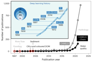
Long-standing challenges in water quality

Water quality has been degrading worldwide under the compound stresses of direct and indirect human influence 23 , including increased pollution loads from urbanization and agricultural expansion 24 , more frequent and prolonged duration of hypoxia in a warming climate 25 , and persistent and widespread harmful algal blooms (HABs) 26 . Understanding and predicting water quality are therefore imperative but have faced major challenges. First, water chemistry is complex and encompasses many variables. For example, the US Geological Survey maintains an inventory of up to 24,898 water-quality variables across 17 categories ( https://help.waterdata.usgs.gov/codes-and-parameters/parameters ). In this Review, we cast a wide but incomplete net by searching the literature for DL modelling of common water-quality term ( Supplementary Text ). Their transport and fate are regulated by interacting, complex processes under distinct environmental conditions. These multiple layers of complexity make it challenging to measure, model, understand and predict water quality.

Challenges with data scarcity

Data collection and measurements are the foundation of scientific discovery. They enable the formulation of hypotheses and the development of conceptual and numerical models. Compared with streamflow, water-quality data, however, are often more sparse, inconsistent, and limited in time, space and frequency 27 (Fig. 1 ), partly owing to the complexity of water-quality variables. Common water-quality measurements include water temperature (WT), total suspended solids (TSS), dissolved oxygen (DO), biological and chemical oxygen demand, salinity, specific conductance, turbidity, sediments, clarity, alkalinity, chlorophyll  a (chl  a ), carbon and nutrients in various forms (for example, dissolved organic carbon, nitrate (NO 3 ), total nitrogen (TN), total phosphorous (TP) and toxic metals (for example, arsenic, lead). Most water-quality variables still require manual and labour-intensive measurements using ‘grab samples’ and chemical analysis using large, complex analytical instruments, in contrast to hydrological data (for example, precipitation, streamflow, evapotranspiration and snow depth) that are often measured automatically 27 . Although sensors have been developed for hundreds of water-quality variables 28 , their in situ deployment for routine, automatic measures are limited in location, duration and water-quality variables (for example, WT, DO, specific conductance, nutrients, dissolved organic carbon). Even for the most abundantly measured TSS, the global average is limited to 29 data counts per station, 1.1% of days with data and a record duration of 4.2 years (Fig. 1 ), compared with 12,066, 84% and 38 years for streamflow. Some sites do have long-term water-quality records, although they are a small fraction of the total (outliers in Supplementary Fig. 1 ).

a , b , Temporal trends of the number of global gauges reporting at least one data point for streamflow ( Q ) ( a ) and water quality ( b ), with data from the Global Streamflow Indices and Metadata Archive (GSIM) 136 and the Global River Water Quality Archive (GRQA) 137 , respectively. The inset maps show global gauge locations. c , d , The outliers in Supplementary Fig. 1 . The 25%, 50% (middle line) and 75% percentiles of data length ( c ) and temporal coverage ( d ). Streamflow Q has a total of 374 million data points from 30,959 sites, whereas TSS has a total of ~2 million data points from 68,592 sites. Other variables include TP (1.9 million data points from 44,943 sites), DO (1.2 million data points from 48,066 sites), NO 3 (1.2 million from 44,551 sites) and particulate organic carbon (POC; 0.62 million data points from 22,877 sites). The length (yr, c ) is the number of years that have data points. The coverage (%, d ) is the temporal coverage percentage with data points in days. Streamflow ( Q ) gauging started in the United States in the 1880s and increased steadily until 1960s 138 , when gauges began to expand across Europe and other continents ( a ). A decrease in streamflow gauges since 2015 may indicate withering investment 139 , or a latency in data mobilization: it takes time for new observations to become publicly available. The first gauge for TSS, the most abundant water-quality variable, was established in the United States in 1898 137 ( b ), almost 20 years after the first streamflow gauge. The spike in observations in the 1970s probably arose from the substantial water infrastructure investments from the Clean Water Act 140 . Noticeable declines followed around 1980 and 1995 are possibly due to funding cuts 141 . Observations in the GLORICH database extend only until 2011 (see breakdown in Supplementary Fig. 2 ), leading to another decline after 2010 ( b ).

In addition, data availability is highly heterogeneous: approximately 83% of global TSS data comes from 17% of the sampled rivers, predominantly in North America. Other variables have even lower coverages (Fig. 1b–d ). An additional limitation of grab samples is that water-quality monitoring often fails to capture the full range of streamflow regimes (for example, transient peak flow), often leading to bias in modelling water quality. Furthermore, monitoring efforts are often patchy, tailored to address specific environmental concerns, such as a summer algal bloom event or metal pollution resulting from a mine-waste spill. These localized, short-term datasets may have limited applicability for broader assessments or long-term trend analyses. Note that most examples in the following section are US based due to the availability of openly accessible, long-term water-quality datasets; however, relevant DL studies in other global locations are discussed wherever possible.

Challenges with model prediction

Predicting water-quality dynamics remains a major challenge yet is essential for water management, risk mitigation and climate adaptation 29 . Linear statistical approaches, including those integrating mass balances, are meaningful screening tools to assess drivers (for example, climate, urbanization, agricultural expansion). They, however, are typically limited by the assumption of linear and/or stationary relationships between drivers, concentrations or loads of focal variables, and therefore cannot simulate changing dynamics and predict future water-quality conditions. Other non-ML statistical models similarly have limited flexibility and adaptability to changing conditions. For example, LoadEST (Load Estimator) 30 and WRTDS (Weighted Regressions on Time, Discharge, and Season) 31 are primarily based on the relationships between concentration, discharge and time. These estimates can be compromised when these relationships vary and depend on unmodelled factors 32 . ML has gained popularity due to its ability to analyse and extract patterns from large and complex datasets without relying on explicit physical or chemical equations. However, traditional ML models often require manual engineering for feature extraction from input data and struggle to capture long-term temporal dependencies in scarce data. This is particularly the case for water-quality data. For example, the global average TSS record duration is 4.2 years per site, far from sufficient for capturing long-term trends.

Process-based models are another model category for water-quality predictions. These models typically solve ordinary or partial differential equations based on mass-balance principles of water and chemical variables and explicitly simulate underlying processes that govern water-quality dynamics. One of their major strengths is to provide insights into mechanisms of water-quality dynamics 33 , as they are guided by physics and chemistry principles. Process-based models, however, suffer from several major limitations. In most cases, we lack a comprehensive, mechanism-based understanding such that processes may not be accurately and adequately represented in the models 34 . Process-based models also require detailed data on a myriad of processes and properties 35 , including above- and below-ground characteristics, water flow, and biogeochemical processes, which are time-consuming and expensive to collect. Process-based models are also computationally expensive, particularly when simulating at large spatio-temporal scales and resolutions. They are also limited because extrapolation from one variable to another often requires different process representation and calibration data, and therefore model re-development or re-calibration, even within the same watershed 33 . This is challenging because water-quality concerns vary by space and time.

Deep learning approaches

Strengths of dl approaches.

DL approaches can provide high predictive accuracy 36 and have the potential to address long-standing challenges facing traditional statistical and process-based models. DL models are flexible, adaptable, integrative, scalable and speedy. They are flexible, in that they can learn complex relationships from raw data without requiring a careful feature engineering of inputs and a detailed understanding of underlying processes 7 , making them useful in deciphering high-dimensional environmental data with poorly understood mechanisms. Second, they are adaptable, in that they can learn from new data without requiring substantial modifications of model structure. For example, the same model can often be used when new water-quality observations or management-relevant datasets become available. They are integrative, as they can extract hidden patterns and nonlinear representations from diverse data sources 8 , such as sensor data, satellite images and grab chemistry data that vary in availability and spatio-temporal coverage. They are scalable as they are designed to learn directly from data that already embed information on spatial and temporal scales 9 , which can reduce the need for model parameters at particular scales that are important yet often unavailable via measurements. Such parameters include, for example, local hyporheic exchange and solute transformation rates. DL models are also speedy, as they take advantage of both hardware advances and optimization algorithms that are designed to efficiently traverse high-dimensional parameter space and converge quickly, enabling the exploration of many environmental scenarios and prediction of many parameters across broad spatial and temporal extents.

In some instances, DL can also represent physical processes in climate and geoscience models, where these processes might be inadequately understood and coarsely modelled 8 , 22 . For example, deep neural networks (DNNs) have been applied to represent turbulent processes in ocean models 37 and atmospheric subgrid processes in climate models 38 to minimize the prohibitive cost of running high-resolution physical models. The saved computational resources can then be reallocated to enhance simulations either by increasing ensemble sizes or by improving the model resolution 39 . These advantages and features, as well as the use of problem-specific DL architectures such as CNN for spatial analysis and RNN for time-series tasks (Box 1 ), are well suited to modelling the complex and spatiotemporally dynamic nature of water-quality conditions.

Limitations of DL approaches

Despite gaining tremendous momentum, DL models have limitations. In addition to requiring significant computational resources such as GPUs and TPUs, DL models require enormous datasets to train effectively. Without sufficient data, they are prone to overfitting 9 . That is, they become too closely tailored to the training data and fail to aptly generalize to new conditions. In other words, DL models are only as good as their data; if they have not seen enough data, for example, under extreme conditions, they cannot learn to extract the input–output relationship under these conditions and are not better than traditional models. In hydrology, the availability of large benchmark datasets (for example, Catchment Attributes and Meteorology for Large-Sample Studies (CAMELS)) has evolved concurrently with fast-growing DL applications (Box 2 ). DL applications in water quality have grown comparatively slowly, potentially indicating data limitations as a bottleneck (Fig. 1 and Box 2 ). DL models are additionally criticized as being ‘black boxes’ and lack interpretability and generalizability, such that it is challenging to understand mechanisms and extrapolate beyond training data. These limitations have triggered advances in PGDL, as discussed in later sections.

Deep learning for data-scarcity challenges

The challenges of data scarcity cannot be resolved overnight. Data collection requires investments in physical and human resources and technological innovations, including the development of new sensors that can automatically measure variables under more frequent and intensifying extreme conditions. Yet the need to understand and predict water quality is urgent as we face pressing water-quality issues under changing climate conditions and human stresses. With ample data, DL models can predict water quality at times and locations without observations (spatial and temporal data filling) and help discover new information through model and data interrogation. In fact, recent work has leveraged publicly available data, including satellite imagery and hydrometeorology data, to predict water quality in surface and subsurface waters with scarce data.

Spatial data filling in chemically ungauged basins

Prediction from well-monitored to ungauged and unmonitored locations has been a long-standing challenge. DL models have recently shown promises in making prediction for chemically ungauged basins. Water-quality data in monitored locations have been used to build models together with hydrometeorological data, remote-sensing data or spatial features such as basin characteristics, and then extrapolate to ungauged rivers. For example, a continental-scale long short-term memory (LSTM) model trained with DO data from 480 US rivers made robust predictions in 100 rivers where data were purposely excluded from the training dataset to resemble ungauged rivers 40 (Fig. 2 ). LSTMs trained with process-based model predictions and WT observations from 145 well-monitored lakes achieved better performance than a pure process-based model of lake temperature when transferred to 1,882 less-monitored lakes in the Midwest United States 41 . A deep gated recurrent unit (GRU) model combined satellite images with relatively limited in situ measurements (that is, 1,260 pairs of water-clarity data from 399 lakes) to infer water clarity in 16,475 global lakes with little or no data 42 . Spatially explicit DL models have filled spatial gaps using the effects of unmonitored reaches on their neighbours to infer water quality at all reaches. Spatial relationships among stream reaches have been represented through graph convolution on an adjacency matrix based on stream distance 43 or travel time 44 for temperature prediction, or even detailed process-based routing within a DL context for streamflow prediction 45 . Such relationships can be made more nuanced by learning more specifics of reaches, such as those with reservoirs and those without 46 or for learned clusters of physically similar reaches 47 .

a – e , A continental-scale LSTM model ( d ) was trained with hydrometeorological data ( a ), sparse DO data ( b ) and constant basin attributes ( c ) from 480 rivers to predict DO dynamics in 100 ‘chemically ungauged basins’ (blank white region with triangles in US map; e ), where data were excluded during training. f , The DL model robustly reproduced the long-term (1980–2019) DO trends and seasonal variations (zoom in) in these ‘data excluded’ rivers, indicating its potential in predicting DO in chemically ungauged basins. In d , X t , C t and h t represent the input, cell state and hidden state at the current timestep t , respectively. The symbols σ and tanh refer to sigmoid and tanh functions, respectively. Pink circles denoted by × and + correspond to point-by-point multiplication and addition operations, respectively. Panels adapted with permission from: a , b , d , ref. 12 , American Chemical Society; e , f , ref. 40 , Springer Nature Ltd.

Temporal data filling

DL models have been used to predict time series of water quality by incorporating spatial features, temporal correlations and nonlinearity without prior assumptions. Such capabilities underscore its potential for effectively filling temporal data gaps. For example, using time series of intensively measured hydrometeorological data, sparse DO data and static watershed characteristics as inputs, a trained LSTM model predicted daily DO in hundreds of US rivers 12 , 40 (Fig. 2 ). A regional multi-site LSTM model reproduced and gap-filled daily NO 3 measurements at 42 monitored stream reaches in Iowa 48 with improved performance (Supplementary Table 1 ). Furthermore, a modified LSTM model 49 combined hydrometeorological data and physical properties of lakes (for example, coordinates, elevation, surface area) and predicted daily WT from 1980 to 2020 in 185,549 US lakes 50 . LSTM models have also used spatial information from adjacent groundwater wells to enhance the accuracy of temporal gap filling for specific conductance, especially for large decadal gaps in the Columbia River 51 . Another study demonstrated that an LSTM model outperformed other ML models (for example, support vector machine, single-layer perceptron) in predicting daily TSS concentrations in a Malaysian river 52 . A hybrid encoder–decoder bidirectional LSTM model showed higher accuracy than ML (extreme gradient boosting) and standalone DL methods in predicting daily sediment loads in the Godavari River Basin in India 53 .

Predicting data-scarce variables from data-rich surrogates

Water chemistry sensors have been increasingly deployed in recent years at temporal resolutions as fine as minutes; they, however, are limited to a handful of variables (for example, turbidity, specific conductance, pH, WT, DO and NO 3 ) with scant spatio-temporal coverage. Most water-quality variables are manually measured at low frequencies (for example, monthly, quarterly). Traditional remote sensing for water quality has primarily focused on optically active variables such as chl  a 54 , coloured dissolved organic matter DOM (DOM) 55 and water clarity 56 in large water bodies (oceans and large lakes and rivers); remote-sensing data often have insufficient spatial resolution for small rivers and streams.

Many water-quality variables, however, are intrinsically linked by shared transport dynamics, redox conditions and biogeochemical processes including, for example, soil respiration and nutrient transformation 57 . These relationships among variables have long been acknowledged and leveraged by surrogate regression models for sediments 58 , pesticides 59 and nutrients 60 , among others. Data-rich variables can therefore provide information about data-poor variables. DL approaches are now beginning to explore this opportunity. For example, DL models have recently been used to estimate nutrients that are non-optically active, based on their correlations with optically active variables that were estimated via remote sensing. A backpropagation neural network model trained with limited measurements and satellite-retrieved sea surface salinity and remote-sensing reflectance successfully estimated NO 3 and phosphate concentrations 61 . Another DL model estimated TN and TP based on their correlations with chl  a and remote-sensing reflectance, and further reconstructed spatio-temporal patterns of nutrients from 1984 to 2020 62 . These estimated variables can further predict other variables, such as dissolved carbon, that are less frequently measured but are essential for water quality, and CO 2 –climate feedbacks 63 . LSTM- and GRU-based models have been used to estimate TP and heavy metal concentrations (that is, copper, zinc) in urban sewer networks from commonly measured variables (for example, temperature, pH, conductivity) 64 , 65 .

Predicting groundwater quality from catchment properties

Earth’s subsurface, or the critical zone from soils to parent bedrock 66 , governs the storage and flow of groundwater, biogeochemical reactions and chemical transport from groundwater to surface waters, and, therefore, surface water quality 67 . The subsurface, however, is not as readily accessible (for example, via boreholes or geophysics), such that below-ground data are even more scarce 68 , 69 .

Subsurface properties and functions are generally not as temporally variable as those at the surface. Deep CNN-based DL models, therefore, are often used to extract spatial patterns. DL models have been shown to outperform traditional calibration approaches in estimating subsurface parameters, because they can directly infer parameters from observations and capture the high nonlinearity with fewer realizations 70 , 71 . For example, a deep CNN-based model recently used two-dimensional land-surface data, including digital elevation maps and remote-sensing images, to construct three-dimensional subsurface structures in an Australian desert landscape 72 . The model revealed complex relationships between surface and subsurface features that are often obscured by traditional methods such as sequential Gaussian. The DL model automated a low-cost method to generate a three-dimensional subsurface structure that inherits the probability structure of a real two-dimensional surface image. Another DNN model used widely available time-series streamflow data to estimate permeability, an essential property that determines flow rates that are arduous to measure directly 73 , outperforming traditional ensemble smoother methods.

Non-DL algorithms have also been used to estimate spatial variations of mean groundwater quality. For example, random forest and generalized boosted regression models have been increasingly applied to predict groundwater contaminants from local to global scales 74 , 75 , 76 , 77 . An ML model trained with groundwater chemistry (for example, alkalinity, Ca, Mg, turbidity) was used to detect anomalous methane in groundwater in areas of shale gas production across the United States 78 . ML models have also been used to fill global gaps of groundwater contaminants including fluoride 75 and arsenic 74 (Fig. 3 ). In fact, groundwater chemistry may be better predicted by ML methods that can explicitly link environmental variables to spatial variability in groundwater chemistry but require fewer data. In many groundwater cases, predicting spatial variation may be more important than temporal trends, because prediction maps can help identify areas of low groundwater quality. Future opportunities lie in developing DL models that can train well with scarce data. For instance, some groundwater solutes may originate from the same geological setting. In these cases, transfer models could be trained on a larger dataset and then used to perform learning on less-measured water-quality variables.

a , Map of 55,000 groundwater arsenic concentrations used as input to ML models. b , A global map of probability of arsenic in groundwater exceeding 10 µg l −1 (ref. 74 ). Some groundwater chemistry does not vary as much as in surface water, such that ML models without time dependence my be sufficient for generating spatial prediction maps. This example shows the potential of data-driven methods in estimating scarce groundwater chemistry. Figure adapted with permission from ref. 74 , AAAS.

Deep learning for robust predictions

A common concern about DL is its limited generalizability, that is, capability to extrapolate beyond the training data 9 . Unlike traditional process-based models, DL models usually rely solely on patterns in training data, which may be scarce especially under climate extremes such as fires, floods and droughts 57 . Advances to improve model performance with existing knowledge primarily reside in two directions: process-guided deep learning (PGDL) and differential modelling (DM). As shown in examples below, most existing applications of PGDL and DM are more in the realm of improving model prediction and parameter estimation. These approaches are expected to reveal process-based understanding and new knowledge but have yet to demonstrate such capabilities. PGDL and DM applications in water quality have been limited so far; we therefore also draw examples from hydrology to illustrate their potential use.

Process-guided deep learning

PGDL seeks to encode domain knowledge within otherwise domain-agnostic model architectures and training algorithms 79 . By doing so, the PGDL model leverages well-established process knowledge and discourages violation of known principles, which also helps earn stakeholder trust such that stakeholders use model outputs more readily. An advantage of PGDL over DL is the improved accuracy and reliability beyond training conditions 80 . PGDL can also improve the physical realism of DL predictions where data are limited, noisy or incomplete. One PGDL approach is to use output from process-based models (not necessarily calibrated) as additional training data 81 , which augments the availability of data. PGDL can also be achieved by using physically meaningful loss function terms, such as a penalty for the lack of mass or energy conservation 82 , 83 , or by adding asymmetric activation functions 84 to enforce constraints imposed by underlying processes, such as flow, transport and energy balance. Loss terms and constraints that explicitly encode hydrological or biogeochemical knowledge may look much like process-based models, with the advantage that the PGDL elements are written in a DL language that provides automatic differentiation, that is, calculation of gradients of outputs relative to all model variables. PGDL thus overlaps with the emerging field of DM, which closely interweaves process-based model equations and neural networks in a single differentiable language 85 . As an example, a hybrid physics-guided RNN model for lake temperature 86 incorporated energy conservation and density–depth relations into the loss function as penalty terms. The model was pretrained using simulated energy budgets from the physics-based General Lake Model to initialize the network structure and fill in scarce data. The model performed better and can project to warmer and colder conditions beyond training data. Similarly, an LSTM model pretrained with an energy budget formulation and WT predictions from the General Lake Model performed robustly when extended to 68 lakes outside of the training conditions 82 .

Some PGDL methods additionally utilize multi-task learning, where DL models are trained to simultaneously predict related variables, such as streamflow and stream temperature, to encourage the learning of process-relevant information shared between variables 87 . For instance, a physics-informed neural network for subsurface solute transport 88 incorporated Darcy’s law and advection–dispersion equations in a DL model and trained it together with hydraulic conductivity, hydraulic head and solute concentrations. The approach predicted concentrations of a synthetic solute that better matched a synthetic dataset than the standard DL model, especially when the training data were sparse. The model accuracy further improved when multiple variables were jointly inverted. Compared with single-task models, jointly predicted stream temperature and flow may have better performance, especially when hyperparameters are carefully tuned 87 .

Differentiable modelling

DM aims to integrate process-based equations with DL models to simultaneously advance process representations, parameter estimation and predictive accuracy 22 . DM encodes existing knowledge and neural networks in an automatically differentiable programming language to reap the advantages of the physical underpinnings of process-based models and the learning capabilities of DL. DM includes physically meaningful parameters and equations that can be inspected and/or manipulated. DM can additionally approach the predictive accuracy of purely data-driven DL, suggesting that the DL components of a DM model can learn relationships that are encoded by process-based components. Recent analyses showed that DM with a physical model as the backbone can outperform pure DL, yielding more accurate regional extrapolation of streamflow with respect to daily metrics and decadal trends 80 . Similarly, embedding the hydrologic model EXP-HYDRO within an RNN structure and augmenting it with neural network layers accurately captured snow water equivalent and transferred streamflow prediction across different rivers 89 . A recent work introduced neural networks to substitute ordinary differential equations for representing hydrologic processes 90 . The results showed comparable performance to DL methods, surpassing a conceptual hydrologic model in streamflow prediction for 569 US rivers while retaining the interpretability of the conceptual model. Furthermore, a process-based model integrated an advective dispersion equation with a river network graph and predicted stream WT more accurately in data-sparse situations 44 .

Deep learning for knowledge discovery

DL approaches have been criticized as being ‘black boxes’ 9 : the algorithms find the optimal combination of layers and weight functions to fit data without offering insights into mechanisms. Such a black-box approach does not reveal its inner workings and new knowledge of processes. With increasing awareness of this limitation, the pursuit of methods to judge the trustworthiness of DL approaches is growing, aiming to turn black boxes into transparent glass boxes for interpretability and knowledge discovery (Fig. 4 ). The toolbox of such techniques is growing 91 . Explainable deep learning (XDL) approaches aim to illuminate the ‘black box’ by evaluating model ‘reasoning’, interpreting model decisions, and extracting patterns and drivers (Fig. 4 ). XDL includes model-agnostic and model-specific approaches that identify and rank important features, relationships and mechanisms that contribute to model predictions 92 . Model-agnostic concepts include integrated gradients 93 , expected gradients 94 , Shapley additive explanations (SHAP) 95 and surrogate models such as local interpretable model-agnostic explanations (LIME) 96 . They do not require a specific model structure and therefore can provide comparable outputs for different models. Model-specific approaches include attention mechanisms, saliency maps and decision trees, and can tailor explanations for specific models (for example, transformers, CNNs and tree-based algorithms, respectively). These techniques elucidate ‘behaviours’ of deep learning 97 , 98 and support hypothesis generation. Hypothesis testing is essential for falsifying assumptions and theories and uncovering potentially overlooked patterns and correlations 99 . Consequently, this process fosters knowledge discovery, enhances process-based understanding, and facilitates more interpretable prediction and informed decision-making.

The efforts include using PGDL (purple), DM and XDL (green) along with revealing visualizations. Domain knowledge can be integrated into DL at various stages, such as selecting important features, pretraining DL models using outputs from process-based models and multi-task learning. Alternatively, process-guided loss functions or differentiable process-based modules (for example, dashed box) can be used to incorporate mass conservation, energy balance, flow transport or other process knowledge to enhance model performance. Knowledge discovery can emerge from accurate predictions themselves, from inspecting variables and learned parameters within the model itself (for example, internal signals), and from XDL. XDL includes common post hoc methods such as integrated gradients (IG), expected gradients (EG), SHAP and LIME, and model-specific methods such as attention mechanisms.

XDL has been used mostly in understanding temporal trends, spatial patterns, and predominant drivers of streamflow, water temperature (WT), and a limited number of water-quality variables. For example, XDL has been used to understand the spatial relationships of stream temperature and the seasonal importance of streamflow versus wind and air pressure in controlling saltwater intrusion into the Delaware River 100 . Saliency maps have been used to highlight the most important regions of an input image for predicting streamflow 98 , suggesting that global sea surface temperatures influence river flows via atmospheric convection and teleconnections. Another study used SHAP values and identified WT, DO and TP as the most influential drivers of riverine chl  a , a widely used indicator of harmful algae blooms (HABs) 101 . A DNN model predicted a variety of water-quality variables, from which SHAP values identified the most influential factors 102 . In addition, hybrid models integrating existing knowledge and DL are promising in potentially advancing both prediction accuracy and process-based understanding. For example, a hybrid model for lake phosphorous combined an RNN model with ecological principles (for example, power scaling) 103 . The model predicted short-term and long-term variations in observed phosphorous with high accuracy, outperforming the process-based model and RNN alone. The model identified lake level and thermocline depth as the most important drivers of phosphorous loads and revealed a decade-long downwards trend as contributing to the long and slow change in phosphorous loads. The model further suggested that including an additional temperature component can improve the process-based model.

The future of deep learning in water quality

As DL becomes increasingly applied, tested and improved in old and new regimes, DL will probably become increasingly trustworthy for predicting future water quality under various management, policy, climate and socioeconomic scenarios. As Earth’s climate evolves, climate extremes such as floods, droughts, cyclones and fires will become more frequent and severe. Such extremes often alter concentrations and loads of sediments and solutes by orders of magnitude 57 , 104 . During extreme wildfires, for example, sediment-loaded water often overwhelms water treatment plants 105 ; during droughts, DO often drops to critically low levels and endangers aquatic ecosystems 106 . Water-quality hindcast and near-term forecasts, therefore, will be essential for designing water infrastructure and making real-time decisions on water and ecosystem management. In addition, the growing challenges of water-quality management will make trustworthy forecasts and scenario projections increasingly valuable. DL can be potentially leveraged not only for extreme events forecasting but also for general management such as identifying pollution sources 107 , optimizing monitoring networks 108 and management decisions 109 , and automatically monitoring water quality 54 , 110 . Such predictions are critical for adapting to climate changes and mitigating the impact of extreme events.

Approaches for hindcasts and forecasts will continue to face challenges of data scarcity and incomplete process understanding, although the approaches described above can begin to ameliorate these challenges. Furthermore, new developments in alternative methods such as Bayesian modelling 111 , evolutionary algorithms 112 and transfer learning 113 , as well as their hybrid use with DL models, could be leveraged for improved prediction. For example, a DL-guided evolutionary algorithm was trained to use sensor data to identify contamination sources and improve computational efficiency and model performance 114 . A transfer-learning-based LSTM model captured the long-term dependencies among time series and leveraged knowledge learned from complete datasets, improving imputation accuracy by 15–25% for DO concentration 115 .

Existing work on water quality, whether using traditional DL, XDL, PGDL or DM, has only scratched the surface of our capacity to learn from DL models. Most work has been limited to a few variables such as WT and DO that are largely influenced by meteorological conditions, sediment and phosphorus that are primarily driven by discharge regimes, as well as optically active variables such as chl  a and coloured DOM that can be directly inferred from the spectral signatures of satellite images. For now, every addition to the literature is valuable in developing our sense of what is possible and how to make the best possible use of DL, not only in practical uses such as forecasting extreme events but also in further developing theories and insights that drive water-quality dynamics.

Prediction for extreme events and climate scenarios

Water management under extreme conditions traditionally relies on human expertise (for example, subjective detection thresholds) and ensemble models for extreme weather prediction. However, models such as LSTM have shown promise in forecasts under extreme conditions with lead times of up to days 116 . As extreme events intensify and alter water quality, traditional process-based models may be limited by our understanding of water-quality theory under extreme conditions 57 . Existing data, if measured under extreme conditions (a big ‘if’ for water quality), may already contain valuable information that surpasses our current understanding 117 . Such hidden knowledge in data can be leveraged in DL models to forecast water quality under extreme conditions. As an example, HABNet, a model that combines CNN and LSTM, has discriminated between HAB and non-HAB events using remote-sensing data, outperforming historical methods 54 . An integrated PGDL and data assimilation approach forecasted daily WT up to 7 days in advance with accuracy and quantified uncertainties 109 , enabling water management decisions such as reservoir water release when WT rose above a fish tolerance threshold.

Such existing work is only the tip of the iceberg. We anticipate that DL-based forecasting will expand beyond algae blooms and WT. The bottleneck of such forecasting is still sufficient data under extreme conditions 118 . To train well, DL models have to see sufficient input to output response to figure out trends and patterns. Extreme conditions challenge data collection, because physical conditions during, for example, floods, often prevent manual data collection but also knock out sensors used for automatic data collection. Extreme events, although predicted to occur more frequently, will still occur less frequently such that the temporal window for monitoring is fleeting. Advances in technology for robust and automatic measurements are essential in both gushing waters and in close-to-zero-flow dry riverbeds 119 .

Predicting the future and projecting hypothetical scenarios into the future demand more than a capability for hindcasts. Data-driven models of all kinds (statistical, ML broadly and DL specifically) may predict accurately on training data but fail spectacularly under new input conditions. Generalizability demands that new conditions we wish to project are represented in the training datasets, which is often not the case. XDL can help evaluate the physical realism of DL predictions under diverse conditions, and PGDL can encourage DL models to encode physically realistic relationships. Rigorous tests of new DL models are needed with respect to generalizability. These include conducting spatio-temporal extrapolation tests in ungauged basin and future (lead) forecast, as well as in benchmark tests against other established methods or models. These tests will offer the capability to represent complex processes and project to new scenarios with more confidence and transparency, supporting decision-makers in anticipating and responding to water-quality challenges. Progress has been made with encouraging preliminary findings 82 , 100 ; DL generalizability, however, should not be taken for granted.

Diversifying data sources to combat data scarcity

The challenges of data scarcity will continue, because data collection requires investment, human resources and innovation. Data scarcity can be ameliorated with expanded use of traditional DL, PGDL and DM in conjunction with observations of surrogates and other biogeochemically related predictors. However, data ‘generated’ by DL-based approaches should be used with caution. Another approach is to leverage an even wider diversity of data sources. For example, hydrology data are much more available than water-quality data. Remote-sensing data, social media data and citizen science data have become widely available. Social media posts, including text, pictures and videos, have been mined for flood-water level estimation 120 , flood assessment 121 and water-quality classification 122 . Citizen science has also become increasingly useful in hydrological and water-quality research 123 , 124 , 125 . Cost-effective crowdsourced monitoring can additionally engage the public, thereby enhancing the long-term sustainability of monitoring networks 123 . For example, community-based monitoring provides water-quality data (for example, pH, WT, electrical conductivity) in Chile 124 and Australia 126 ( https://www.waterwatch.org.au ). Citizen science data, however, may be challenging for water-quality variables, as measurements of most solutes require expensive technology and changes in solute concentrations are often invisible. Yet they can potentially provide ‘complementary’ information on environmental conditions or human behaviour for DL models to learn, infer and forecast water quality.

Seeking new knowledge

Earth’s subsurface governs water storage, transport and the generation of water-quality variables via biogeochemical reactions 127 , therefore regulating the chemistry of subsurface source water that eventually enters rivers and lakes 57 . In fact, a significant portion of surface waters derive from soil water and groundwater 128 . Surface water chemistry therefore reflects water flow paths and its interactions with soils, rocks, microbes and roots that mobilize solutes and sediments 129 . Existing theories and empirical relationships abound depicting how physical, chemical and biological processes mobilize solids and solutes 40 , 43 , 130 . Simultaneous use of both process-based and DL models, whether independently or within a coupled framework, can inspire new hypotheses about mechanisms and drivers of water-quality dynamics (Fig. 4 ).

XDL tools can potentially be used to compare PGDL and non-PGDL models and reveal what the models can learn differently when we ask and/or enable them to better conform to a physics-based reality. Interrogating XDL of multi-task models may reveal influential predictors or latent variables the models learn to produce and share among multiple variables. The learned relationships can further generate hypotheses. Theories and process-based equations combined with DL modules in the DM framework may also enable rapid calibration and comparison of competing process representations for hypothesis testing 22 . In addition, model interrogation with different types of input can reveal influential drivers. For example, assessment of model performance with different inputs have revealed temperature as the predominant driver of daily DO in US rivers 40 . Robust model training offers consistent ‘data’ output with filled gaps, which can enable extraction of temporal trends and spatial patterns. For example, a multi-task LSTM model trained on WT and DO data in about 800 rivers revealed that rivers warm up most rapidly in urban rivers and lose oxygen most rapidly in agricultural rivers, and that they lose oxygen faster than oceans 131 . These approaches could open doors for knowledge discovery.

The opportunities for combined XDL, PGDL and DM to inform knowledge exist, although they have yet to realize their full potential. Current DL research has focused more on approaches and model performance than on knowledge discovery. The emerging data (whether original observation or model filled) and knowledge from these approaches can have far-reaching impacts, not only on water-quality prediction but also on broad understanding of processes that shape global biogeochemical cycles of carbon, nutrients and other elements, and climate feedbacks 132 .

In summary, while transparent, interpretable process-based and statistical models will remain important for predicting water quality, DL models can potentially overcome long-standing data limitations and predictive challenges inherent to these traditional approaches. DL approaches, however, are only as robust as the quality and quantity of the available data. Data and observations are the bedrock of all scientific discoveries 133 , 134 . Without intercepted messages, Turing could not have decoded Enigma 135 . Similar to children learning to speak, DL models must ‘see’ or ‘hear’ enough data to decipher hidden patterns and laws. Using diverse data sources, including remote sensing, social media content, citizen science data, surrogate water-quality measurements and process-based model outputs, can potentially improve our ability to leverage DL for understanding and predicting water quality. Despite these additional sources, data availability will probably remain the bottleneck of DL applications in water quality. Paradoxically, with the ‘right’ amount of data, DL models can help predict water quality in time and space, filling data gaps and reconstructing long-term data. A potential future direction is to integrate DL and process-based models (for example, PGDL, DM), harnessing their individual merits for improved prediction, transparency, and knowledge discovery.

We predict that the emergent power of DL approaches for improving global water quality will be realized through: (1) collating publicly available spatial and temporal data and exploring their relationships with water-quality variables for spatio-temporal prediction; (2) bringing new tools and fresh eyes to discover hidden patterns, processes and relationships that regulate water-quality dynamics; and 3) predicting future and unmonitored water-quality conditions to explore options for managing and mitigating water-quality impairments under climate extremes, and broadly in a rapidly changing world. The outcome could have far-reaching impacts not only in water-quality fields but also broadly in understanding and predicting the future of global cycles of carbon, nutrients, other elements and beyond.

Data availability

Streamflow data (Fig. 1a ) from the Global Streamflow Indices and Metadata Archive (GSIM) were compiled from repositories at https://doi.org/10.1594/PANGAEA.887477 and https://doi.org/10.1594/PANGAEA.887470 . Water-quality data (Fig. 1b ) from the Global River Water Quality Archive (GRQA) were downloaded from https://doi.org/10.5281/zenodo.7056647 .

Turing, A. M. Computing machinery and intelligence. Mind 59 , 433–460 (1950).

Article   Google Scholar  

Turing, A. M. On computable numbers, with an application to the Entscheidungsproblem. Proc. Lond. Math. Soc. s2-42 , 230–265 (1937).

Muggleton, S. Alan Turing and the development of artificial intelligence. AI Commun. 27 , 3–10 (2014).

Dechter, R. Learning while searching in constraint-satisfaction problems. In Proceedings of the AAAI Conference on Artificial Intelligence Vol. 5, 178–183 (AAAI, 1986).

Hinton, G. E. & Salakhutdinov, R. R. Reducing the dimensionality of data with neural networks. Science 313 , 504–507 (2006).

Article   CAS   PubMed   Google Scholar  

Hinton, G. E., Osindero, S. & Teh, Y.-W. A fast learning algorithm for deep belief nets. Neural Comput. 18 , 1527–1554 (2006).

Article   PubMed   Google Scholar  

Lecun, Y., Bengio, Y. & Hinton, G. Deep learning. Nature 521 , 436–444 (2015).

Reichstein, M. et al. Deep learning and process understanding for data-driven Earth system science. Nature 566 , 195–204 (2019).

Shen, C. A transdisciplinary review of deep learning research and its relevance for water resources scientists. Water Resour. Res. 54 , 8558–8593 (2018).

Shen, C. P. et al. HESS opinions: incubating deep-learning-powered hydrologic science advances as a community. Hydrol. Earth Syst. Sci. 22 , 5639–5656 (2018).

Xu, T. & Liang, F. Machine learning for hydrologic sciences: an introductory overview. Wiley Interdiscip. Rev. Water 8 , e1533 (2021).

Zhi, W. et al. From hydrometeorology to river water quality: can a deep learning model predict dissolved oxygen at the continental scale? Environ. Sci. Technol. 55 , 2357–2368 (2021).

Varadharajan, C. et al. Can machine learning accelerate process understanding and decision‐relevant predictions of river water quality? Hydrol. Process. https://doi.org/10.1002/hyp.14565 (2022).

Tripathy, K. P. & Mishra, A. K. Deep learning in hydrology and water resources disciplines: concepts, methods, applications, and research directions. J. Hydrol. https://doi.org/10.1016/j.jhydrol.2023.130458 (2023).

Perry, G. L. W., Seidl, R., Bellvé, A. M. & Rammer, W. An outlook for deep learning in ecosystem science. Ecosystems 25 , 1700–1718 (2022).

Song, T. et al. A review of artificial intelligence in marine science. Front. Earth Sci. https://doi.org/10.3389/feart.2023.1090185 (2023).

Sun, A. Y. & Scanlon, B. R. How can big data and machine learning benefit environment and water management: a survey of methods, applications, and future directions. Environ. Res. Lett. 14 , 073001 (2019).

Zhu, J.-J., Yang, M. & Ren, Z. J. Machine learning in environmental research: common pitfalls and best practices. Environ. Sci. Technol. 57 , 17671–17689 (2023).

van Klompenburg, T., Kassahun, A. & Catal, C. Crop yield prediction using machine learning: a systematic literature review. Comput. Electron. Agric. 177 , 105709 (2020).

Zhong, S. et al. Machine learning: new ideas and tools in environmental science and engineering. Environ. Sci. Technol. https://doi.org/10.1021/acs.est.1c01339 (2021).

Appling, A. P., Oliver, S. K., Read, J. S., Sadler, J. M. & Zwart, J. A. in Encyclopedia of Inland Waters 2nd edn (eds Mehner, T. & Tockner, K.) 585–606 (Elsevier, 2022).

Shen, C. et al. Differentiable modelling to unify machine learning and physical models for geosciences. Nat. Rev. Earth Environ. 4 , 552–567 (2023).

Diamond, J. S. et al. Hypoxia is common in temperate headwaters and driven by hydrological extremes. Ecol. Indic. 147 , 109987 (2023).

Article   CAS   Google Scholar  

Creed, I. F. et al. Enhancing protection for vulnerable waters. Nat. Geosci. 10 , 809–815 (2017).

Article   CAS   PubMed   PubMed Central   Google Scholar  

Nazari-Sharabian, M., Ahmad, S. & Karakouzian, M. Climate change and eutrophication: a short review. Eng. Technol. Appl. Sci. Res. 8 , 3668 (2018).

Paerl, H. W., Otten, T. G. & Kudela, R. Mitigating the expansion of harmful algal blooms across the freshwater-to-marine continuum. Environ. Sci. Technol. 52 , 5519–5529 (2018).

McCabe, M. F. et al. The future of Earth observation in hydrology. Hydrol. Earth Syst. Sci. 21 , 3879–3914 (2017).

Article   PubMed   PubMed Central   Google Scholar  

Abbott, B. W. et al. Using multi-tracer inference to move beyond single-catchment ecohydrology. Earth Sci. Rev. 160 , 19–42 (2016).

Milly, P. C. D. et al. Stationarity is dead: whither water management? Science 319 , 573–574 (2008).

Runkel, R. L., Crawford, C. G. & Cohn, T. A. Load Estimator (LOADEST): A FORTRAN Program for Estimating Constituent Loads in Streams and Rivers Report no. 4-A5 (USGS, 2004).

Hirsch, R. M., Moyer, D. L. & Archfield, S. A. Weighted regressions on time, discharge, and season (WRTDS), with an application to Chesapeake Bay River inputs. J. Am. Water Resour. Assoc. 46 , 857–880 (2010).

Zhang, Q., Blomquist, J. D., Moyer, D. L. & Chanat, J. G. Estimation bias in water-quality constituent concentrations and fluxes: a synthesis for Chesapeake Bay rivers and streams. Front. Ecol. Evol. https://doi.org/10.3389/fevo.2019.00109 (2019).

Zhi, W. et al. Distinct source water chemistry shapes contrasting concentration–discharge patterns. Water Resour. Res. 55 , 4233–4251 (2019).

Archfield, S. A. et al. Accelerating advances in continental domain hydrologic modeling. Water Resour. Res. 51 , 10078–10091 (2015).

Zhi, W. et al. BioRT-Flux-PIHM v1.0: a watershed biogeochemical reactive transport model. Geosci. Model Dev. 15 , 19 (2022).

Rahmani, F. et al. Exploring the exceptional performance of a deep learning stream temperature model and the value of streamflow data. Environ. Res. Lett. https://doi.org/10.1088/1748-9326/abd501 (2021).

Bolton, T. & Zanna, L. Applications of deep learning to ocean data inference and subgrid parameterization. J. Adv. Model. Earth Syst. 11 , 376–399 (2019).

Rasp, S., Pritchard, M. S. & Gentine, P. Deep learning to represent subgrid processes in climate models. Proc. Natl Acad. Sci. USA 115 , 9684–9689 (2018).

Irrgang, C. et al. Towards neural Earth system modelling by integrating artificial intelligence in Earth system science. Nat. Mach. Intell. 3 , 667–674 (2021).

Zhi, W., Ouyang, W., Shen, C. & Li, L. Temperature outweighs light and flow as the predominant driver of dissolved oxygen in US rivers. Nat. Water 1 , 249–260 (2023).

Willard, J. D. et al. Predicting water temperature dynamics of unmonitored lakes with meta-transfer learning. Water Resour. Res. 57 , e2021WR029579 (2021).

He, Y. et al. Water clarity mapping of global lakes using a novel hybrid deep-learning-based recurrent model with Landsat OLI images. Water Res. 215 , 118241 (2022).

Jia, X. et al. Physics-guided recurrent graph model for predicting flow and temperature in river networks. In Proc. 2021 SIAM International Conference on Data Mining (SDM) 612–620 (SIAM, 2021); https://doi.org/10.1137/1.9781611976700.69

Bao, T. et al. Partial differential equation driven dynamic graph networks for predicting stream water temperature. In 2021 IEEE International Conference on Data Mining (ICDM) 11–20 (IEEE, 2021); https://doi.org/10.1109/ICDM51629.2021.00011

Bindas, T. et al. Improving river routing using a differentiable Muskingum‐Cunge model and physics‐informed machine learning. Water Resour. Res. 60 , e2023WR035337 (2024).

Chen, S. et al. Heterogeneous stream-reservoir graph networks with data assimilation. In 2021 IEEE International Conference on Data Mining (ICDM) 1024–1029 (IEEE, 2021).

Chen, S., Zwart, J. A. & Jia, X. Physics-guided graph meta learning for predicting water temperature and streamflow in stream networks. In Proc. 28th ACM SIGKDD Conference on Knowledge Discovery and Data Mining 2752–2761 (Association for Computing Machinery, 2022).

Saha, G. K., Rahmani, F., Shen, C., Li, L. & Cibin, R. A deep learning-based novel approach to generate continuous daily stream nitrate concentration for nitrate data-sparse watersheds. Sci. Total Environ. 878 , 162930 (2023).

Kratzert, F. et al. Towards learning universal, regional, and local hydrological behaviors via machine learning applied to large-sample datasets. Hydrol. Earth Syst. Sci. 23 , 5089–5110 (2019).

Willard, J. D., Read, J. S., Topp, S., Hansen, G. J. A. & Kumar, V. Daily surface temperatures for 185,549 lakes in the conterminous United States estimated using deep learning (1980–2020). Limnol. Oceanogr. Lett. https://doi.org/10.1002/lol2.10249 (2022).

Ren, H., Cromwell, E., Kravitz, B. & Chen, X. Using long short-term memory models to fill data gaps in hydrological monitoring networks. Hydrol. Earth Syst. Sci. 26 , 1727–1743 (2022).

Latif, S. D. et al. Sediment load prediction in Johor River: deep learning versus machine learning models. Appl. Water Sci. https://doi.org/10.1007/s13201-023-01874-w (2023).

Jamei, M. et al. Designing a decomposition-based multi-phase pre-processing strategy coupled with EDBi-LSTM deep learning approach for sediment load forecasting. Ecol. Indic. 153 , 110478 (2023).

Hill, P. R., Kumar, A., Temimi, M. & Bull, D. R. HABNet: machine learning, remote sensing-based detection of harmful algal blooms. IEEE J. Sel. Top. Appl. Earth Obs. Remote Sens. 13 , 3229–3239 (2020).

D’Alimonte, D., Zibordi, G. & Berthon, J. F. Determination of CDOM and NPPM absorption coefficient spectra from coastal water remote sensing reflectance. IEEE Trans. Geosci. Remote Sens. 42 , 1770–1777 (2004).

Zhang, Y. et al. Improving remote sensing estimation of Secchi disk depth for global lakes and reservoirs using machine learning methods. GIsci. Remote Sens. 59 , 1367–1383 (2022).

Li, L. et al. River water quality shaped by land–river connectivity in a changing climate. Nat. Clim. Change https://doi.org/10.1038/s41558-023-01923-x (2024).

Rasmussen, P. P., Gray, J. R., Glysson, G. D. & Ziegler, A. C. Guidelines and Procedures for Computing Time-Series Suspended-Sediment Concentrations and Loads from In-Stream Turbidity-Sensor and Streamflow Report No. 3-C4 (USGS, 2009).

Covert, S. A., Bunch, A. R., Crawford, C. G. & Oelsner, G. P. Comparison of Surrogate Models to Estimate Pesticide Concentrations at Six U.S. Geological Survey National Water Quality Network Sites during Water Years 2013–18 Report No. 2022-5109 (USGS, 2023).

Schilling, K. E., Kim, S.-W. & Jones, C. S. Use of water quality surrogates to estimate total phosphorus concentrations in Iowa rivers. J. Hydrol. Reg. Stud. 12 , 111–121 (2017).

Wang, D. et al. Satellite retrieval of surface water nutrients in the coastal regions of the East China Sea. Remote Sens. 10 , 1896 (2018).

Guo, H. et al. Performance of deep learning in mapping water quality of Lake Simcoe with long-term Landsat archive. ISPRS J. Photogramm. Remote Sens. 183 , 451–469 (2022).

Kerins, D. & Li, L. High dissolved carbon concentration in arid rocky mountain streams. Environ. Sci. Technol. 57 , 4656–4667 (2023).

Zhang, Y. et al. A hybrid model combining mode decomposition and deep learning algorithms for detecting TP in urban sewer networks. Appl. Energy 333 , 120600 (2023).

Jiang, Y., Li, C., Song, H. & Wang, W. Deep learning model based on urban multi-source data for predicting heavy metals (Cu, Zn, Ni, Cr) in industrial sewer networks. J. Hazard. Mater. https://doi.org/10.1016/j.jhazmat.2022.128732 (2022).

Li, L. et al. Expanding the role of reactive transport models in critical zone processes. Earth Sci. Rev. 165 , 280–301 (2017).

Li, L. et al. Toward catchment hydro-biogeochemical theories. WIREs Water 8 , e1495 (2021).

Bergen, K. J., Johnson, P. A., de Hoop, M. V. & Beroza, G. C. Machine learning for data-driven discovery in solid Earth geoscience. Science 363 , eaau0323 (2019).

Kolbe, T. et al. Stratification of reactivity determines nitrate removal in groundwater. Proc. Natl Acad. Sci. USA 116 , 2494–2499 (2019).

Sun, A. Y. Discovering state‐parameter mappings in subsurface models using generative adversarial networks. Geophys. Res. Lett. https://doi.org/10.1029/2018gl080404 (2018).

Jiang, P., Shuai, P., Sun, A., Mudunuru, M. K. & Chen, X. Knowledge-informed deep learning for hydrological model calibration: an application to Coal Creek Watershed in Colorado. Hydrol. Earth Syst. Sci. Discuss. 2022 , 1–31 (2022).

Google Scholar  

Jiang, Z. et al. Sub3DNet1.0: a deep-learning model for regional-scale 3D subsurface structure mapping. Geosci. Model Dev. 14 , 3421–3435 (2021).

Cromwell, E. et al. Estimating watershed subsurface permeability from stream discharge data using deep neural networks. Front. Earth Sci. https://doi.org/10.3389/feart.2021.613011 (2021).

Podgorski, J. & Berg, M. Global threat of arsenic in groundwater. Science 368 , 845–850 (2020).

Podgorski, J. & Berg, M. Global analysis and prediction of fluoride in groundwater. Nat. Commun. https://doi.org/10.1038/s41467-022-31940-x (2022).

Ransom, K. M., Nolan, B. T., Stackelberg, P. E., Belitz, K. & Fram, M. S. Machine learning predictions of nitrate in groundwater used for drinking supply in the conterminous United States. Sci. Total Environ. 807 , 151065 (2022).

Nolan, B. T., Green, C. T., Juckem, P. F., Liao, L. & Reddy, J. E. Metamodeling and mapping of nitrate flux in the unsaturated zone and groundwater, Wisconsin, USA. J. Hydrol. 559 , 428–441 (2018).

Wen, T., Liu, M., Woda, J., Zheng, G. & Brantley, S. L. Detecting anomalous methane in groundwater within hydrocarbon production areas across the United States. Water Res. 200 , 117236 (2021).

Willard, J., Jia, X., Xu, S., Steinbach, M. & Kumar, V. Integrating scientific knowledge with machine learning for engineering and environmental systems. ACM Comput. Surv. 55 , 1–37 (2023).

Feng, D., Beck, H., Lawson, K. & Shen, C. The suitability of differentiable, learnable hydrologic models for ungauged regions and climate change impact assessment. Hydrol. Earth Syst. Sci. Discuss. 2022 , 1–28 (2022).

Sun, A. Y., Yoon, H., Shih, C.-Y. & Zhong, Z. Applications of physics-informed scientific machine learning in subsurface science: A survey. In Knowledge Guided Machine Learning (eds Karpatne, A. et al.) 111–132 (Chapman and Hall/CRC, 2022).

Read, J. S. et al. Process‐guided deep learning predictions of lake water temperature. Water Resour. Res. 55 , 9173–9190 (2019).

Beucler, T., Rasp, S., Pritchard, M. & Gentine, P. Achieving conservation of energy in neural network emulators for climate modeling. Preprint at https://arxiv.org/abs/1906.06622 (2019).

Daw, A. et al. Physics-Guided Architecture (PGA) of Neural Networks for Quantifying Uncertainty in Lake Temperature Modeling. In Proc. 2020 SIAM International Conference on Data Mining (SDM) 532–540 (SIAM, 2020).

Shen, C. et al. Differentiable modelling to unify machine learning and physical models for geosciences. Nat. Rev. Earth Environ. https://doi.org/10.1038/s43017-023-00450-9 (2023).

Jia, X. et al. Physics Guided RNNs for Modeling Dynamical Systems: A Case Study in Simulating Lake Temperature Profiles. In Proceedings of the 2019 SIAM International Conference on Data Mining 558–566 (SIAM, 2019).

Sadler, J. M. et al. Multi-task deep learning of daily streamflow and water temperature. Water Resour. Res. 58 , e2021WR030138 (2022).

He, Q., Barajas-Solano, D., Tartakovsky, G. & Tartakovsky, A. M. Physics-informed neural networks for multiphysics data assimilation with application to subsurface transport. Adv. Water Res. 141 , 103610 (2020).

Jiang, S., Zheng, Y. & Solomatine, D. Improving AI system awareness of geoscience knowledge: symbiotic integration of physical approaches and deep learning. Geophys. Res. Lett. https://doi.org/10.1029/2020gl088229 (2020).

Höge, M., Scheidegger, A., Baity-Jesi, M., Albert, C. & Fenicia, F. Improving hydrologic models for predictions and process understanding using neural ODEs. Hydrol. Earth Syst. Sci. 26 , 5085–5102 (2022).

Molnar, C. Interpretable Machine Learning (Lulu.com, 2020).

Samek, W., Montavon, G., Lapuschkin, S., Anders, C. J. & Muller, K.-R. Explaining deep neural networks and beyond: a review of methods and applications. Proc. IEEE 109 , 247–278 (2021).

Sundararajan, M., Taly, A. & Yan, Q. Axiomatic attribution for deep networks. In International Conference on Machine Learning 3319–3328 (ICML, 2017).

Erion, G. et al. Improving performance of deep learning models with axiomatic attribution priors and expected gradients. Nat. Mach. Intell. 3 , 620–631 (2021).

Lundberg, S. M. & Lee, S.-I. A unified approach to interpreting model predictions. Adv. Neural Inf. Process. Syst. 30 , 1–10 (2017).

Ribeiro, M. T., Singh, S. & Guestrin, C. " Why should i trust you?" Explaining the predictions of any classifier. In Proc. 22nd ACM SIGKDD International Conference on Knowledge Discovery and Data Mining 1135–1144 (ACM, 2016).

Xie, W. et al. Interpretable framework of physics‐guided neural network with attention mechanism: simulating paddy field water temperature variations. Water Resour. Res. 58 , e2021WR030493 (2022).

Liu, Y., Duffy, K., Dy, J. G. & Ganguly, A. R. Explainable deep learning for insights in El Niño and river flows. Nat. Commun. https://doi.org/10.1038/s41467-023-35968-5 (2023).

Sadayappan, K., Kerins, D., Shen, C. & Li, L. Nitrate concentrations predominantly driven by human, climate, and soil properties in US rivers. Water Res. 226 , 119295 (2022).

Topp, S. N. et al. Stream temperature prediction in a shifting environment: explaining the influence of deep learning architecture. Water Resour. Res. https://doi.org/10.1029/2022wr033880 (2023).

Lee, D. et al. Integrated explainable deep learning prediction of harmful algal blooms. Technol. Forecast. Soc. Change 185 , 122046 (2022).

Zheng, H., Liu, Y., Wan, W., Zhao, J. & Xie, G. Large-scale prediction of stream water quality using an interpretable deep learning approach. J. Environ. Manage. 331 , 117309 (2023).

Hanson, P. C. et al. Predicting lake surface water phosphorus dynamics using process-guided machine learning. Ecol. Modell. 430 , 109136 (2020).

Carpenter, S. R., Booth, E. G. & Kucharik, C. J. Extreme precipitation and phosphorus loads from two agricultural watersheds. Limnol. Oceanogr. 63 , 1221–1233 (2018).

Robinne, F.-N. et al. Scientists’ warning on extreme wildfire risks to water supply. Hydrol. Process. 35 , e14086 (2021).

Whitehead, P. G., Wilby, R. L., Battarbee, R. W., Kernan, M. & Wade, A. J. A review of the potential impacts of climate change on surface water quality. Hydrol. Sci. J. 54 , 101–123 (2009).

Wang, P. et al. Exploring the application of artificial intelligence technology for identification of water pollution characteristics and tracing the source of water quality pollutants. Sci. Total Environ. 693 , 133440 (2019).

Kontos, Y. N., Kassandros, T., Katsifarakis, K. L. & Karatzas, K. Deep Learning Modeling of Groundwater Pollution Sources. In International Conference on Engineering Applications of Neural Networks 165–177 (Springer, 2021).

Zwart, J. A. et al. Near-term forecasts of stream temperature using deep learning and data assimilation in support of management decisions. J. Am. Water Res. Assoc. 59 , 317–337 (2023).

van Lieshout, C., van Oeveren, K., van Emmerik, T. & Postma, E. Automated river plastic monitoring using deep learning and cameras. Earth Space Sci. 7 , e2019EA000960 (2020).

Beria, H., Larsen, J. R., Michelon, A., Ceperley, N. C. & Schaefli, B. HydroMix v1.0: a new Bayesian mixing framework for attributing uncertain hydrological sources. Geosci. Model Dev. 13 , 2433–2450 (2020).

Tang, Y., Reed, P. & Wagener, T. How effective and efficient are multiobjective evolutionary algorithms at hydrologic model calibration? Hydrol. Earth Syst. Sci. 10 , 289–307 (2006).

Iman, M., Arabnia, H. R. & Rasheed, K. A review of deep transfer learning and recent advancements. Technologies 11 , 40 (2023).

Qian, K., Jiang, J., Ding, Y. & Yang, S.-H. DLGEA: a deep learning guided evolutionary algorithm for water contamination source identification. Neural Comput. Appl. 33 , 11889–11903 (2021).

Chen, Z. et al. A transfer learning-based LSTM strategy for imputing large-scale consecutive missing data and its application in a water quality prediction system. J. Hydrol. 602 , 126573 (2021).

Xiang, Z., Yan, J. & Demir, I. A rainfall-runoff model with LSTM-based sequence-to-sequence learning. Water Resour. Res. 56 , e2019WR025326 (2020).

Nearing, G. S. et al. What role does hydrological science play in the age of machine learning? Water Resour. Res . https://doi.org/10.1029/2020WR028091 (2021).

Guo, D. et al. A data-based predictive model for spatiotemporal variability in stream water quality. Hydrol. Earth Syst. Sci. 24 , 827–847 (2020).

Zimmer, M. A. et al. Zero or not? Causes and consequences of zero-flow stream gage readings. WIREs Water 7 , e1436 (2020).

Chaudhary, P., D’Aronco, S., Moy de Vitry, M., Leitão, J. P. & Wegner, J. D. Flood-water level estimation from social media images. ISPRS Ann. Photogramm. Remote Sens. Spatial Inf. Sci . https://doi.org/10.5194/isprs-annals-IV-2-W5-5-2019 (2019).

Kanth, A. K., Chitra, P. & Sowmya, G. G. Deep learning-based assessment of flood severity using social media streams. Stoch. Environ. Res. Risk Assess. 36 , 473–493 (2022).

Hanif, M., Khawar, A., Tahir, M. A. & Rafi, M. Deep learning based framework for classification of water quality in social media data. In Proc. MediaEval 2021 Workshop ( MediaEval 2021).

Njue, N. et al. Citizen science in hydrological monitoring and ecosystem services management: state of the art and future prospects. Sci. Total Environ. 693 , 133531 (2019).

Yevenes, M. A., Pereira, H. & Bermudez, R. Citizen science as a co-creative measure to water quality: chemical data and local participation in a rural territory. Front. Environ. Sci. 10 , 940778 (2022).

Nardi, F. et al. Citizens and Hydrology (CANDHY): conceptualizing a transdisciplinary framework for citizen science addressing hydrological challenges. Hydrol. Sci. J. 67 , 2534–2551 (2022).

Dyer, F. et al. Waterwatch data quality: an opportunity to augment professionally collected data sets. In Proc. 7th Australian Stream Management Conference 27–30 (ASM, 2014).

Rose, L. A., Karwan, D. L. & Godsey, S. E. Concentration–discharge relationships describe solute and sediment mobilization, reaction, and transport at event and longer timescales. Hydrol. Processes 32 , 2829–2844 (2018).

Hare, D. K., Helton, A. M., Johnson, Z. C., Lane, J. W. & Briggs, M. A. Continental-scale analysis of shallow and deep groundwater contributions to streams. Nat. Commun. https://doi.org/10.1038/s41467-021-21651-0 (2021).

Li, L. et al. Toward catchment hydro‐biogeochemical theories. WIREs Water https://doi.org/10.1002/wat2.1495 (2021).

Zhi, W. & Li, L. The shallow and deep hypothesis: subsurface vertical chemical contrasts shape nitrate export patterns from different land uses. Environ. Sci. Technol. 54 , 11915–11928 (2020).

Zhi, W., Klingler, C., Liu, J. & Li, L. Widespread deoxygenation in warming rivers. Nat. Clim. Change 13 , 1105–1113 (2023).

Li, L. et al. Climate controls on river chemistry. Earths Future 10 , e2021EF002603 (2022).

Harari, Y. N. Sapiens: A Brief History of Humankind (Random House, 2014).

Popper, K. The Logic of Scientific Discovery (Basic Books, 1959).

Hodges, A. Alan Turing: The Enigma: The Centenary Edition (Princeton Univ. Press, 2012).

Do, H. X., Gudmundsson, L., Leonard, M. & Westra, S. The Global Streamflow Indices and Metadata Archive (GSIM)—Part 1: the production of a daily streamflow archive and metadata. Earth Syst. Sci. Data 10 , 765–785 (2018).

Virro, H., Amatulli, G., Kmoch, A., Shen, L. & Uuemaa, E. GRQA: global river water quality archive. Earth System Sci. Data 13 , 5483–5507 (2021).

Gunn, M. A., Matherne, A. M. & Mason, J. R. R. The USGS at Embudo, New Mexico: 125 Years of Systematic Streamgaging in the United States Report No. 2014-30344 (USGS, 2014).

Burt, T. P. & McDonnell, J. J. Whither field hydrology? The need for discovery science and outrageous hydrological hypotheses. Water Resour. Res. 51 , 5919–5928 (2015).

Read, E. K. et al. Water quality data for national‐scale aquatic research: the Water Quality Portal. Water Resour. Res. 53 , 1735–1745 (2017).

Council, N. R. Confronting the Nation’s Water Problems: The Role of Research (National Academies Press, 2004).

Li, Z., Liu, H., Zhang, C. & Fu, G. Generative adversarial networks for detecting contamination events in water distribution systems using multi-parameter, multi-site water quality monitoring. Environ. Sci. Ecotechnol. 14 , 100231 (2023).

Qu, H. & Yuan, W. Water quality Anomaly detection based on optimally reconfigured convolutional autoencoder. In 2022 International Conference on Wearables, Sports and Lifestyle Management (WSLM) 137–141 (IEEE, 2022).

Shen, C., Chen, X. & Laloy, E. Broadening the use of machine learning in hydrology. Front. Water https://doi.org/10.3389/frwa.2021.681023 (2021).

Schmidhuber, J. Annotated history of modern AI and deep learning. Preprint at https://arxiv.org/abs/2212.11279 (2022).

McCulloch, W. S. & Pitts, W. A logical calculus of the ideas immanent in nervous activity. Bull. Math. Biophys. 5 , 115–133 (1943).

Rosenblatt, F. The perceptron: a probabilistic model for information storage and organization in the brain. Psychol. Rev. 65 , 386 (1958).

Amari, S.-I. Learning patterns and pattern sequences by self-organizing nets of threshold elements. IEEE Trans. Comput. 100 , 1197–1206 (1972).

Maier, H. R. & Dandy, G. C. The use of artificial neural networks for the prediction of water quality parameters. Water Resour. Res. 32 , 1013–1022 (1996).

Maier, H. R. & Dandy, G. C. Neural networks for the prediction and forecasting of water resources variables: a review of modelling issues and applications. Environ. Modell. Softw. 15 , 101–124 (2000).

Chang, F. J. & Hwang, Y. Y. A self-organization algorithm for real-time flood forecast. Hydrol. Process. 13 , 123–138 (1999).

Dawson, C. W. & Wilby, R. L. A comparison of artificial neural networks used for river flow forecasting. Hydrol. Earth Syst. Sci. 3 , 529–540 (1999).

Cigizoglu, H. K. Estimation and forecasting of daily suspended sediment data by multi-layer perceptrons. Adv. Water Res. 27 , 185–195 (2004).

Dransfeld, S., Tatnall, A. R., Robinson, I. S. & Mobley, C. D. A comparison of multi-layer perceptron and multilinear regression algorithms for the inversion of synthetic ocean colour spectra. Int. J. Remote Sens. 25 , 4829–4834 (2004).

Pankiewicz, G. S. Neural network classification of convective airmasses for a flood forecasting system. Int. J. Remote Sens. 18 , 887–898 (1997).

Addor, N., Newman, A. J., Mizukami, N. & Clark, M. P. The CAMELS data set: catchment attributes and meteorology for large-sample studies. Hydrol. Earth Syst. Sci. 21 , 5293–5313 (2017).

Newman, A. et al. Development of a large-sample watershed-scale hydrometeorological data set for the contiguous USA: data set characteristics and assessment of regional variability in hydrologic model performance. Hydrol. Earth Syst. Sci. 19 , 209 (2015).

Kratzert, F. et al. Caravan—a global community dataset for large-sample hydrology. Sci. Data https://doi.org/10.1038/s41597-023-01975-w (2023).

GEMStat Database of the Global Environment Monitoring System for Freshwater (GEMS/Water) Programme (UN Environment Programme, 2018).

Hartmann, J., Lauerwald, R. & Moosdorf, N. GLORICH—global river chemistry database. Pangaea 902360 , 520 (2019).

Rotteveel, L., Heubach, F. & Sterling, S. M. The Surface Water Chemistry (SWatCh) database: a standardized global database of water chemistry to facilitate large-sample hydrological research. Earth Syst. Sci. Data 14 , 4667–4680 (2022).

Sterle, G. et al. CAMELS-Chem: augmenting CAMELS (Catchment Attributes and Meteorology for Large-sample Studies) with atmospheric and stream water chemistry data. Hydrol. Earth Syst. Sci. Discuss. 2022 , 1–23 (2022).

D’Alimonte, D. & Zibordi, G. Phytoplankton determination in an optically complex coastal region using a multilayer perceptron neural network. IEEE Trans. Geosci. Remote Sens. 41 , 2861–2868 (2003).

Download references

Acknowledgements

W.Z. was supported by the National Natural Science Foundation of China (52121006) and by the Barry and Shirley Isett Professorship (to L.L.) at Penn State University. L.L. was supported by the US National Science Foundation via the Critical Zone Collaborative Network (EAR-2012123 and EAR-2012669), Frontier Research in Earth Sciences (EAR-2121621), Signals in Soils (EAR-2034214), and US Department of Energy Environmental System Science (DE-SC0020146). J.P. was supported by Swiss Agency for Development and Cooperation (SDC) (WABES project, 7F-09963.02.01). This paper has been reviewed in accordance with the US Environmental Protection Agency’s peer and administrative review policies and approved for publication. Mention of trade names or commercial products does not constitute endorsement or recommendation for use. Any use of trade, firm, or product names is for descriptive purposes only and does not imply endorsement or recommendation for use by the US Government. Statements in this publication reflect the authors’ professional views and opinions and should not be construed to represent any determination or policy of the US Environmental Protection Agency.

Author information

Authors and affiliations.

The National Key Laboratory of Water Disaster Prevention, Yangtze Institute for Conservation and Development, Key Laboratory of Hydrologic-Cycle and Hydrodynamic-System of Ministry of Water Resources, Hohai University, Nanjing, China

Department of Civil and Environmental Engineering, The Pennsylvania State University, University Park, PA, USA

Wei Zhi & Li Li

US Geological Survey, Reston, VA, USA

Alison P. Appling

Office of Research and Development, US Environmental Protection Agency, Cincinnati, OH, USA

Heather E. Golden

Department of Water Resources and Drinking Water, Swiss Federal Institute of Aquatic Science and Technology (EAWAG), Dübendorf, Switzerland

Joel Podgorski

You can also search for this author in PubMed   Google Scholar

Contributions

W.Z. and L.L. conceived the idea for the review paper and wrote the first draft. A.P.A., H.E.G. and J.P. provided content for multiple sections and edited multiple versions of the paper. L.L. finalized the paper.

Corresponding author

Correspondence to Li Li .

Ethics declarations

Competing interests.

The authors declare no competing interests.

Peer review

Peer review information.

Nature Water thanks Danlu Guo and the other, anonymous, reviewer(s) for their contribution to the peer review of this work.

Additional information

Publisher’s note Springer Nature remains neutral with regard to jurisdictional claims in published maps and institutional affiliations.

Supplementary information

Supplementary information.

Supplementary text, Figs. 1 and 2, and Table 1.

Rights and permissions

Springer Nature or its licensor (e.g. a society or other partner) holds exclusive rights to this article under a publishing agreement with the author(s) or other rightsholder(s); author self-archiving of the accepted manuscript version of this article is solely governed by the terms of such publishing agreement and applicable law.

Reprints and permissions

About this article

Cite this article.

Zhi, W., Appling, A.P., Golden, H.E. et al. Deep learning for water quality. Nat Water 2 , 228–241 (2024). https://doi.org/10.1038/s44221-024-00202-z

Download citation

Received : 13 April 2023

Accepted : 10 January 2024

Published : 12 March 2024

Issue Date : March 2024

DOI : https://doi.org/10.1038/s44221-024-00202-z

Share this article

Anyone you share the following link with will be able to read this content:

Sorry, a shareable link is not currently available for this article.

Provided by the Springer Nature SharedIt content-sharing initiative

Quick links

• Explore articles by subject
• Guide to authors
• Editorial policies

Sign up for the Nature Briefing newsletter — what matters in science, free to your inbox daily.

share this!

March 28, 2024

This article has been reviewed according to Science X's editorial process and policies . Editors have highlighted the following attributes while ensuring the content's credibility:

fact-checked

peer-reviewed publication

trusted source

New approach to monitoring freshwater quality can identify sources of pollution, predict their effects

by University of Cambridge

The source of pollutants in rivers and freshwater lakes can now be identified using a comprehensive new water quality analysis, according to scientists at the University of Cambridge and Trent University, Canada.

Microparticles from car tires , pesticides from farmers' fields, and toxins from harmful algal blooms are just some of the organic chemicals that can be detected using the new approach, which also indicates the impact these chemicals are likely to have in a particular river or lake.

Importantly, the approach can also point to the origin of specific organic matter dissolved in the water, because it has a distinct composition depending on its source.

It uses a technique called high-resolution mass spectrometry to analyze water samples : within an hour this provides a comprehensive overview of all the organic molecules present. The paper is published in the journal Science .

Water quality is strongly determined by the diversity of organic matter dissolved in it—termed "chemodiversity." The scientists say that the thousands of different dissolved organic compounds can keep freshwater ecosystems healthy, or contribute to their decline, depending on the mixture present.

"Traditional approaches to monitoring water quality involve taking lots of different measurements with many devices, which takes a lot of time. Our technique is a very simple way to get a comprehensive overview of what's going on in a particular river or lake," said Jérémy Fonvielle, a researcher in the University of Cambridge's Department of Biochemistry and co-author of the paper.

To understand what drives this chemodiversity, the team reviewed studies of dissolved organic matter in freshwater samples from rivers and lakes across Europe and northern Canada.

For example, water analysis of Lake Erie in Canada revealed high levels of phosphorus pollution. By looking at the composition of individual molecules in the water sample, researchers identified agricultural activities as the source of this pollution, rather than wastewater effluent.

"Whereas before, we could measure the amount of organic nitrogen or phosphorus pollution in a river, we couldn't really identify where pollution was coming from. With our new approach we can use the unique molecular fingerprint of different sources of pollution in freshwater to identify their source," said Dr. Andrew Tanentzap at Trent University School of the Environment, co-author of the report.

Traditional approaches involve separately measuring many indicators of ecosystem health, such as the level of organic nutrients or particular pollutants like nitrogen. These can indicate the condition of the water, but not why this state has arisen.

Dissolved organic matter is one of the most complex mixtures on Earth. It consists of thousands of individual molecules, each with their own unique properties. This matter influences many processes in rivers and lakes, including nutrient cycling , carbon storage, light absorption, and food web interactions—which together determine ecosystem function.

Sources of dissolved organic matter in freshwater include urban runoff, agricultural runoff, aerosols and wildfires.

"It's possible to monitor the health of freshwater through the diversity of compounds that are present. Our approach can, and is, being rolled out across the UK," said Tanentzap.

Fonvielle will now apply this technique to analyzing water samples from farmland drainage ditches in the Fens, as part of a project run by the University of Cambridge's Center for Landscape Regeneration to understand freshwater health in this agricultural landscape.

Journal information: Science

Provided by University of Cambridge

Explore further

Feedback to editors

Rock sampled by NASA's Perseverance embodies why rover came to Mars

10 minutes ago

More social birds are more adventurous feeders, study finds

24 minutes ago

New tools reveal how genes work and cells organize

33 minutes ago

Study gives first view of centromere variation and evolution

Criollo cattle: Could an old breed be the beef industry's answer to climate change?

SLAC completes construction of the largest digital camera ever built for astronomy

34 minutes ago

New discovery unravels malaria invasion mechanism

Easy compression, easy flow: Research team designs new granular materials

Researchers closer to near real-time disaster monitoring

Novel fabrication technique takes transition metal telluride nanosheets from lab to mass production

55 minutes ago

Relevant PhysicsForums posts

Major earthquakes - 7.4 (7.2) mag and 6.4 mag near hualien, taiwan.

2 hours ago

Iceland warming up again - quakes swarming

Mar 30, 2024

Unlocking the Secrets of Prof. Verschure's Rosetta Stones

Mar 29, 2024

‘Our clouds take their orders from the stars,’ Henrik Svensmark on cosmic rays controlling cloud cover and thus climate

Mar 27, 2024

Higher Chance to get Lightning Strike by Large Power Consumption?

Mar 20, 2024

A very puzzling rock or a pallasite / mesmosiderite or a nothing burger

Mar 16, 2024

More from Earth Sciences

Related Stories

Study finds chemodiversity of soil-dissolved organic matter altered by microplastics

Jan 19, 2024

Faster growth may help bacteria remove lake plastic waste: study

Jul 30, 2022

Climate change could double greenhouse gas emissions from freshwater lakes

Nov 18, 2019

How aromatic dissolved organic matter affects organic micropollutant adsorption

Mar 7, 2024

River pollution is causing harmful outbreaks of sewage fungus in the UK

Mar 4, 2024

Study finds changing dissolved organic carbon in Maine lakes key to maintaining drinking water quality

Apr 17, 2019

Recommended for you

Research reveals pre-collapse monitoring of Kakhovka Dam, Ukraine

Why artificial submarine curtains won't save West Antarctica's retreating glaciers

California leads US emissions of sulfuryl fluoride: State emits more than rest of country combined, study finds

7 hours ago

A new estimate of US soil organic carbon to improve Earth system models

19 hours ago

Spain's giant hail event worsened by marine heat waves, study finds

Apr 2, 2024

Let us know if there is a problem with our content

Use this form if you have come across a typo, inaccuracy or would like to send an edit request for the content on this page. For general inquiries, please use our contact form . For general feedback, use the public comments section below (please adhere to guidelines ).

Please select the most appropriate category to facilitate processing of your request

Thank you for taking time to provide your feedback to the editors.

Your feedback is important to us. However, we do not guarantee individual replies due to the high volume of messages.

E-mail the story

Your email address is used only to let the recipient know who sent the email. Neither your address nor the recipient's address will be used for any other purpose. The information you enter will appear in your e-mail message and is not retained by Phys.org in any form.

Newsletter sign up

Get weekly and/or daily updates delivered to your inbox. You can unsubscribe at any time and we'll never share your details to third parties.

More information Privacy policy

Donate and enjoy an ad-free experience

We keep our content available to everyone. Consider supporting Science X's mission by getting a premium account.

E-mail newsletter

New approach to monitoring freshwater quality can identify sources of pollution, and predict their effects

The source of pollutants in rivers and freshwater lakes can now be identified using a comprehensive new water quality analysis, according to scientists at the University of Cambridge and Trent University, Canada.

Microparticles from car tyres, pesticides from farmers' fields, and toxins from harmful algal blooms are just some of the organic chemicals that can be detected using the new approach, which also indicates the impact these chemicals are likely to have in a particular river or lake.

Importantly, the approach can also point to the origin of specific organic matter dissolved in the water, because it has a distinct composition depending on its source.

It uses a technique called high-resolution mass spectrometry to analyse water samples: within an hour this provides a comprehensive overview of all the organic molecules present.

Water quality is strongly determined by the diversity of organic matter dissolved in it -- termed 'chemodiversity.' The scientists say that the thousands of different dissolved organic compounds can keep freshwater ecosystems healthy, or contribute to their decline, depending on the mixture present.

The paper is published today in the journal Science .

"Traditional approaches to monitoring water quality involve taking lots of different measurements with many devices, which takes a lot of time. Our technique is a very simple way to get a comprehensive overview of what's going on in a particular river or lake," said Jérémy Fonvielle, a researcher in the University of Cambridge's Department of Biochemistry and co-author of the paper.

To understand what drives this chemodiversity, the team reviewed studies of dissolved organic matter in freshwater samples from rivers and lakes across Europe and northern Canada.

For example, water analysis of Lake Erie in Canada revealed high levels of phosphorus pollution. By looking at the composition of individual molecules in the water sample, researchers identified agricultural activities as the source of this pollution, rather than wastewater effluent.

"Whereas before, we could measure the amount of organic nitrogen or phosphorus pollution in a river, we couldn't really identify where pollution was coming from. With our new approach we can use the unique molecular fingerprint of different sources of pollution in freshwater to identify their source," said Dr Andrew Tanentzap at Trent University School of the Environment, co-author of the report.

Traditional approaches involve separately measuring many indicators of ecosystem health, such as the level of organic nutrients or particular pollutants like nitrogen. These can indicate the condition of the water, but not why this state has arisen.

Dissolved organic matter is one of the most complex mixtures on Earth. It consists of thousands of individual molecules, each with their own unique properties. This matter influences many processes in rivers and lakes, including nutrient cycling, carbon storage, light absorption, and food web interactions -- which together determine ecosystem function.

Sources of dissolved organic matter in freshwater include urban runoff, agricultural runoff, aerosols and wildfires.

"It's possible to monitor the health of freshwater through the diversity of compounds that are present. Our approach can, and is, being rolled out across the UK," said Tanentzap.

Fonvielle will now apply this technique to analysing water samples from farmland drainage ditches in the Fens, as part of a project run by the University of Cambridge's Centre for Landscape Regeneration to understand freshwater health in this agricultural landscape.

• Organic Chemistry
• Nature of Water
• Air Quality
• Air Pollution
• Biodiversity
• Organic farming
• Organic chemistry
• Organic farming methods
• Eutrophication

Story Source:

Materials provided by University of Cambridge . The original text of this story is licensed under a Creative Commons Attribution-NonCommercial-ShareAlike 4.0 International License . Note: Content may be edited for style and length.

Journal Reference :

• Andrew J. Tanentzap, Jérémy A. Fonvielle. Chemodiversity in freshwater health . Science , 2024; 383 (6690): 1412 DOI: 10.1126/science.adg8658

Cite This Page :

Explore More

• Australia On Track for Decades-Long Megadroughts
• Speed of Visual Perception Ranges Widely
• 3D Printed Replica of an Adult Human Ear
• Extremely Fast Wound Healing: New Treatment
• Micro-Lisa! Novel Nano-Scale Laser Writing
• Simple Brain-Computer Link: Gaming With Thoughts
• Clinical Reasoning: Chatbot Vs Physicians
• Understanding People Who Can't Visualize
• Illuminating Oxygen's Journey in the Brain
• DNA Study IDs Descendants of George Washington

Trending Topics

Strange & offbeat.

The Effects of Climate Change

The effects of human-caused global warming are happening now, are irreversible for people alive today, and will worsen as long as humans add greenhouse gases to the atmosphere.

• We already see effects scientists predicted, such as the loss of sea ice, melting glaciers and ice sheets, sea level rise, and more intense heat waves.
• Scientists predict global temperature increases from human-made greenhouse gases will continue. Severe weather damage will also increase and intensify.

Earth Will Continue to Warm and the Effects Will Be Profound

Global climate change is not a future problem. Changes to Earth’s climate driven by increased human emissions of heat-trapping greenhouse gases are already having widespread effects on the environment: glaciers and ice sheets are shrinking, river and lake ice is breaking up earlier, plant and animal geographic ranges are shifting, and plants and trees are blooming sooner.

Effects that scientists had long predicted would result from global climate change are now occurring, such as sea ice loss, accelerated sea level rise, and longer, more intense heat waves.

The magnitude and rate of climate change and associated risks depend strongly on near-term mitigation and adaptation actions, and projected adverse impacts and related losses and damages escalate with every increment of global warming.

Intergovernmental Panel on Climate Change

Some changes (such as droughts, wildfires, and extreme rainfall) are happening faster than scientists previously assessed. In fact, according to the Intergovernmental Panel on Climate Change (IPCC) — the United Nations body established to assess the science related to climate change — modern humans have never before seen the observed changes in our global climate, and some of these changes are irreversible over the next hundreds to thousands of years.

Scientists have high confidence that global temperatures will continue to rise for many decades, mainly due to greenhouse gases produced by human activities.

The IPCC’s Sixth Assessment report, published in 2021, found that human emissions of heat-trapping gases have already warmed the climate by nearly 2 degrees Fahrenheit (1.1 degrees Celsius) since 1850-1900. 1 The global average temperature is expected to reach or exceed 1.5 degrees C (about 3 degrees F) within the next few decades. These changes will affect all regions of Earth.

The severity of effects caused by climate change will depend on the path of future human activities. More greenhouse gas emissions will lead to more climate extremes and widespread damaging effects across our planet. However, those future effects depend on the total amount of carbon dioxide we emit. So, if we can reduce emissions, we may avoid some of the worst effects.

The scientific evidence is unequivocal: climate change is a threat to human wellbeing and the health of the planet. Any further delay in concerted global action will miss the brief, rapidly closing window to secure a liveable future.

Here are some of the expected effects of global climate change on the United States, according to the Third and Fourth National Climate Assessment Reports:

Future effects of global climate change in the United States:

U.S. Sea Level Likely to Rise 1 to 6.6 Feet by 2100

Global sea level has risen about 8 inches (0.2 meters) since reliable record-keeping began in 1880. By 2100, scientists project that it will rise at least another foot (0.3 meters), but possibly as high as 6.6 feet (2 meters) in a high-emissions scenario. Sea level is rising because of added water from melting land ice and the expansion of seawater as it warms. Image credit: Creative Commons Attribution-Share Alike 4.0

Climate Changes Will Continue Through This Century and Beyond

Global climate is projected to continue warming over this century and beyond. Image credit: Khagani Hasanov, Creative Commons Attribution-Share Alike 3.0

Hurricanes Will Become Stronger and More Intense

Scientists project that hurricane-associated storm intensity and rainfall rates will increase as the climate continues to warm. Image credit: NASA

More Droughts and Heat Waves

Droughts in the Southwest and heat waves (periods of abnormally hot weather lasting days to weeks) are projected to become more intense, and cold waves less intense and less frequent. Image credit: NOAA

Longer Wildfire Season

Warming temperatures have extended and intensified wildfire season in the West, where long-term drought in the region has heightened the risk of fires. Scientists estimate that human-caused climate change has already doubled the area of forest burned in recent decades. By around 2050, the amount of land consumed by wildfires in Western states is projected to further increase by two to six times. Even in traditionally rainy regions like the Southeast, wildfires are projected to increase by about 30%.

Changes in Precipitation Patterns

Climate change is having an uneven effect on precipitation (rain and snow) in the United States, with some locations experiencing increased precipitation and flooding, while others suffer from drought. On average, more winter and spring precipitation is projected for the northern United States, and less for the Southwest, over this century. Image credit: Marvin Nauman/FEMA

Frost-Free Season (and Growing Season) will Lengthen

The length of the frost-free season, and the corresponding growing season, has been increasing since the 1980s, with the largest increases occurring in the western United States. Across the United States, the growing season is projected to continue to lengthen, which will affect ecosystems and agriculture.

Global Temperatures Will Continue to Rise

Summer of 2023 was Earth's hottest summer on record, 0.41 degrees Fahrenheit (F) (0.23 degrees Celsius (C)) warmer than any other summer in NASA’s record and 2.1 degrees F (1.2 C) warmer than the average summer between 1951 and 1980. Image credit: NASA

Arctic Is Very Likely to Become Ice-Free

Sea ice cover in the Arctic Ocean is expected to continue decreasing, and the Arctic Ocean will very likely become essentially ice-free in late summer if current projections hold. This change is expected to occur before mid-century.

U.S. Regional Effects

Climate change is bringing different types of challenges to each region of the country. Some of the current and future impacts are summarized below. These findings are from the Third 3 and Fourth 4 National Climate Assessment Reports, released by the U.S. Global Change Research Program .

• Northeast. Heat waves, heavy downpours, and sea level rise pose increasing challenges to many aspects of life in the Northeast. Infrastructure, agriculture, fisheries, and ecosystems will be increasingly compromised. Farmers can explore new crop options, but these adaptations are not cost- or risk-free. Moreover, adaptive capacity , which varies throughout the region, could be overwhelmed by a changing climate. Many states and cities are beginning to incorporate climate change into their planning.
• Northwest. Changes in the timing of peak flows in rivers and streams are reducing water supplies and worsening competing demands for water. Sea level rise, erosion, flooding, risks to infrastructure, and increasing ocean acidity pose major threats. Increasing wildfire incidence and severity, heat waves, insect outbreaks, and tree diseases are causing widespread forest die-off.
• Southeast. Sea level rise poses widespread and continuing threats to the region’s economy and environment. Extreme heat will affect health, energy, agriculture, and more. Decreased water availability will have economic and environmental impacts.
• Midwest. Extreme heat, heavy downpours, and flooding will affect infrastructure, health, agriculture, forestry, transportation, air and water quality, and more. Climate change will also worsen a range of risks to the Great Lakes.
• Southwest. Climate change has caused increased heat, drought, and insect outbreaks. In turn, these changes have made wildfires more numerous and severe. The warming climate has also caused a decline in water supplies, reduced agricultural yields, and triggered heat-related health impacts in cities. In coastal areas, flooding and erosion are additional concerns.

1. IPCC 2021, Climate Change 2021: The Physical Science Basis , the Working Group I contribution to the Sixth Assessment Report, Cambridge University Press, Cambridge, UK.

2. IPCC, 2013: Summary for Policymakers. In: Climate Change 2013: The Physical Science Basis. Contribution of Working Group I to the Fifth Assessment Report of the Intergovernmental Panel on Climate Change [Stocker, T.F., D. Qin, G.-K. Plattner, M. Tignor, S.K. Allen, J. Boschung, A. Nauels, Y. Xia, V. Bex and P.M. Midgley (eds.)]. Cambridge University Press, Cambridge, United Kingdom and New York, NY, USA.

3. USGCRP 2014, Third Climate Assessment .

4. USGCRP 2017, Fourth Climate Assessment .

Related Resources

A Degree of Difference

So, the Earth's average temperature has increased about 2 degrees Fahrenheit during the 20th century. What's the big deal?

What’s the difference between climate change and global warming?

“Global warming” refers to the long-term warming of the planet. “Climate change” encompasses global warming, but refers to the broader range of changes that are happening to our planet, including rising sea levels; shrinking mountain glaciers; accelerating ice melt in Greenland, Antarctica and the Arctic; and shifts in flower/plant blooming times.

Is it too late to prevent climate change?

Humans have caused major climate changes to happen already, and we have set in motion more changes still. However, if we stopped emitting greenhouse gases today, the rise in global temperatures would begin to flatten within a few years. Temperatures would then plateau but remain well-elevated for many, many centuries.

Discover More Topics From NASA

Explore Earth Science

Earth Science in Action

Earth Science Data

Facts About Earth